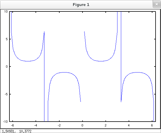
This page shows how to set the graphing window (a.k.a. viewing window) for plots in our favorite CASs.
The axis() command can be used to set the viewing window on the current axes. You may use the syntax axis( [xmin xmax ymin ymax] ) as illustrated below. For details and options of this command consult the documentation.
Simply adding the line axis( [-2*pi 2*pi -10 10] ); to our original attempt to plot $\csc{x}$ for $x\in [-2\pi, 2\pi]$ yields a marked improvement.
octave:1> x = linspace(-2*pi, 2*pi, 81); octave:2> y = csc(x); octave:3> plot( x, y ); octave:4> axis( [-2*pi 2*pi -10 10] );
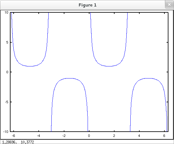
Better yet. Avoid the (infinite) jump discontinuities as demonstrated previously and set the viewing window with axis().
octave:1> eps = 0.0001; % Distance by which we'll avoid singularities octave:2> x = linspace( -2*pi+eps, -pi-eps, 50 ); octave:3> y = csc(x); octave:4> plot( x, y ); octave:5> hold on octave:6> x = linspace( -pi+eps, -eps, 50 ); octave:7> y = csc(x); octave:8> plot( x, y ); octave:9> x = linspace( eps, pi-eps, 50 ); octave:10> y = csc(x); octave:11> plot( x, y ); octave:12> x = linspace( pi+eps, 2*pi-eps, 50 ); octave:13> y = csc(x); octave:14> plot( x, y ); octave:15> axis([-2*pi 2*pi -10 10]);
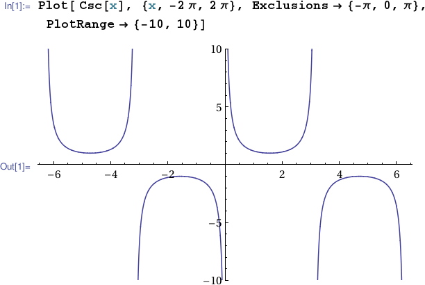
Mathematica tends to choose a reasonable scale on a plot's output axis by default.

But of course the default behavior can be overridden "manually" if desired. The most straightforward way to do this is by setting the PlotRange option.
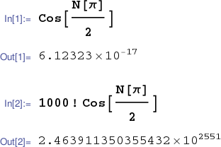
Incidentally, the constant $\pi$ can be entered in a Mathematica notebook with the keyboard sequence Escp Esc or by clicking on the $\pi$ button in the Basic Math Assistant palette. Alternatively you can use Pi (with a capital "P"). Mathematica does not, by default, replace $\pi$ by a numerical approximation, but rather performs exact computations with $\pi$ as a symbolic constant. (If you need to coerce a conversion to a numerical approximation you can enter N[Pi] or Pi//N.) This stands in contrast to MATLAB and GNU Octave where pi is by definition a floating point approximation to $\pi$. Compare, for instance, the Mathematica symbolic computations

with the Octave numerical computations
octave:1> cos(pi/2) ans = 6.1232e-17 octave:2> factorial(1000) * cos(pi/2) ans = Inf.
Forcing Mathematica to working numerically (on my platform) yields
 .
.
The output range for a Sage plot can be set by assigning the desired values to ymin and ymax in the plot() command.
Incidentally Sage, by default, treats pi as an exact mathematical constant. You can obtain a numerical approximation by entering RealField(100)(pi) or n(pi,100).