This page show how to plot more than one function on a single pair of axes. Some new plotting methods are introduced and some inequalities involving trigonometric functions are illustrated. The last Sage interact illustrates the circular function definitions of the six trigonometric functions.
The previously introduced hold on command can be used to combine the plots of more than one function. Often, however, it's more convenient to simply pass more than one pair of input and output arrays in a single invocation of the basic plot command. For example,
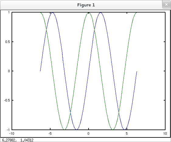
octave:1> x = -2*pi: pi/20 : 2*pi; octave:2> y1 = sin(x); octave:3> y2 = cos(x); octave:4> plot( x, y1, x, y2 )
produces
The assignment x = -2*pi: pi/20 : 2*pi; stores an array of values from $-2\pi$ to $2\pi$ evenly spaced by $\frac{\pi}{20}$ in variable x. This array has 81 values. If you'd prefer to specify the number of values in the array rather than the spacing between consecutive values, you can use the linspace command in place of the colon operator. The syntax for this command is linspace( initial value, final value, number of values), so x = linspace(-2*pi, 2*pi, 81) is equivalent to x = -2*pi: pi/20 : 2*pi.
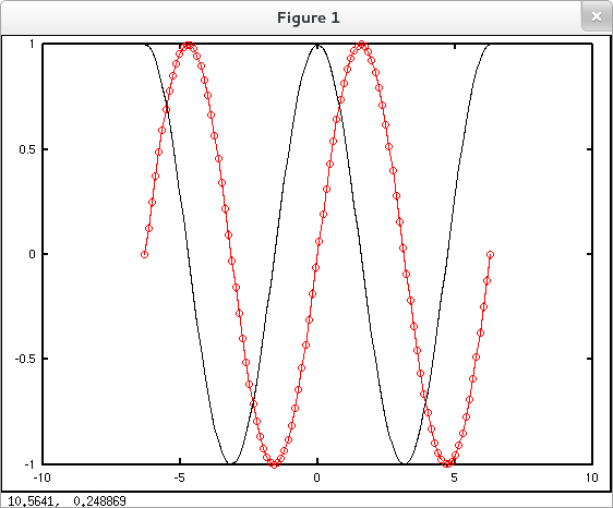
The plot command accepts optional arguments that specify line styles, markers and colors for each plot. Consult Octave or MATLAB documentation for details. For a simple example, the code immediately below plots $\sin{x}$ in red with circular markers next to $\cos{x}$ in black without markers.
octave:1> x = linspace(-2*pi, 2*pi, 100); octave:2> y1 = sin(x); octave:3> y2 = cos(x); octave:4> plot( x, y1, '-or', x, y2, 'k' )
The plotting techniques described so far, applied carelessly, can produce unexpected or undesired results. Consider for example the following attempt to plot the cosecant function on the interval $[-2\pi, 2\pi]$.
octave:1> x = linspace(-2*pi, 2*pi, 81); octave:2> y = csc(x); octave:3> plot( x, y )
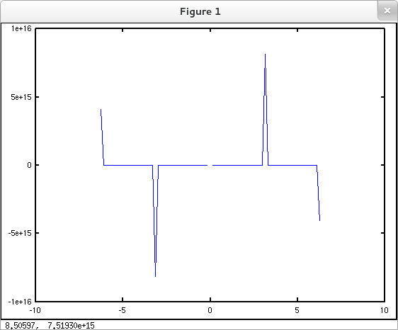
What went wrong? The input array contains five problematic values: an exact representation of $0$ as well as numerical approximations to $\pm\pi$ and $\pm 2\pi$. At $0$, csc evaluates to Inf (infinity) which can't be plotted... accounting for the gap in the middle of the plot, while at the approximations to integer multiples of $\pi$ the function evaluates to finite, but monstrously large values (on the order of $10^{16}$). Scaling the plot to include such huge outputs effectively squashes everything else. The next section discusses graphing windows and demonstrates how you can exercise fine control over the region included in a plot. But for the moment we'll take the "E-Z" way out by looking at the ezplot convenience function. The ezplot command takes an expression depending on variable $x$ and plots it over $[-2\pi, 2\pi]$. (The input interval can be altered from the default $[-2\pi, 2\pi]$ if desired.) This command tends to produce "sane" results.
octave:1> ezplot('csc(x)')

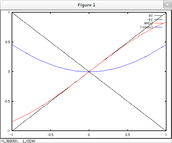
The following sequence of commands plots $\pm|x|$ (in black), $\sin{x}$ (in red), and $1-\cos{x}$ (in blue) over $[-1,1]$ on one set of axes and adds a legend to the plot. The red and blue plots are bounded above and below by the black plots illustrating the inequalities $-|x|\leq \sin{x}\leq |x|$ and $-|x|\leq 1-\cos{x}\leq |x|$.
octave:1> x = linspace(-1,1,100); octave:2> y1 = abs(x); octave:3> y2 = -abs(x); octave:4> y3 = sin(x); octave:5> y4 = 1-cos(x); octave:6> plot( x, y1, 'k', x, y2, 'k', x, y3, 'r', x, y4, 'b' ) octave:7> legend('|x|', '-|x|', 'sin(x)', '1-cos(x)')
Note that although GNU Octave aims to be functionally equivalent to MATLAB, some MATLAB features are not implemented and others produce results which are not precisely the same. If I enter the code above in MATLAB rather than Octave on my system, the legend is added to the plot in a slightly more elegant and readable fashion.
The Mathematica notebook session below shows that Plot[]
accepts a (curly-brace delimited) list of functions to be graphed over
a common interval. Like many other Mathematica commands, Plot[]
accepts optional arguments which modify its behavior. In Mathematica,
optional arguments are entered after required arguments in the form
OptionName -> DesiredValue.
(The keyboard
pair -> (hyphen greater-than) is automatically typeset as an arrow
as appears in the screenshot below.)
Notice that the PlotLegends
package needs to be loaded into the notebook session before the PlotLegends
option may be used.
The plot generated in this example illustrates the inequalities $-|x|\leq \sin{x}\leq |x|$ and $-|x|\leq 1-\cos{x}\leq |x|$.

The plot() command accepts a (parenthesis delimited) list of functions to be graphed over a common interval as in the example below.
In idiomatic Sage complicated plots are often built in stages. Evaluate the following Sage cell to generate an illustration of the inequalities $-|x|\leq\sin{x}\leq |x|$ and $-|x|\leq 1-\cos{x}\leq |x|$.
For fun, let's add a zoom slider. (Slide right to zoom out, and left to zoom in.)
The following interact illustrates the so-called "circular function" definitions of the 6 trig functions. (Notice that the $\theta$ slider uses degrees, not radians.)
.