A function $f$ from set $D$ to set $C$ is a rule that maps each element $x$ in $D$ (the domain) to a unique element $f(x)$ in $C$ (the codomain or target space). Domain elements may be called inputs, while codomain elements that are mapped to may be called outputs. Although an expression defining the output $f(x)$ that a function $f$ produces given a "generic" input $x$ is often itself (imprecisely) referred to as a function, it's useful to recognize the conceptual distinction between the function $f$ and the output $f(x)$ corresponding to input $x$. Without a mastery of this distinction your ability to use CASs effectively (not to mention your progress in higher mathematics) will be handicapped. If someone says, "Let's graph the function $x^2$," you need not pedantically correct them with "You mean, let's graph the function that takes $x$ to $x^2$ (for such-and-such $x$)," or "You mean, let's graph the squaring function," but do be precise when writing mathematical proofs and coding in MATLAB. Otherwise you may lose points on your math exams and run into syntax errors instead of achieving mathematical enlightenment and working, useful programs. This page includes a very brief introduction to the syntax for functions in GNU Octave, MATLAB, Mathematica and Sage. This page also includes an introduction to some of the most basic methods of producing graphs in these CASs.
Suppose you need to work with the function that maps each $x$ in $\mathbb{R}$ to $3|x|-7x+2$. Entering @(x) 3*abs(x) - 7*x + 2 in MATLAB (or Octave) produces a corresponding so-called anonymous function. (Strictly speaking the domain of this anonymous function is not $\mathbb{R}$... but let's not worry about that now.) In Octave you can feed inputs to this function, triggering the system to compute the corresponding outputs as illustrated below.
octave:1> ( @(x) 3*abs(x) - 7*x + 2 )(0) ans = 2 octave:2> ( @(x) 3*abs(x) - 7*x + 2 )(2) ans = -6 octave:3> ( @(x) 3*abs(x) - 7*x + 2 )(-3) ans = 32
Better yet. Use the assignment statement f = @(x) 3*abs(x) - 7*x + 2; (in Octave or MATLAB) to store a so-called handle to the anonymous function in variable f. The function can now be invoked via this handle.
octave:1> f = @(x) 3*abs(x) - 7*x + 2; octave:2> f(0) ans = 2 octave:3> f(2) ans = -6 octave:4> f(-3) ans = 32 octave:5> f([0 2 -3]) ans = 2 -6 32
Contrast the syntax we just used with the following failures.
octave:1> f = 3*abs(x) - 7*x + 2; error: `x' undefined near line 1 column 11 error: evaluating argument list element number 1 octave:1> f(x) = 3*abs(x) - 7*x + 2; error: `x' undefined near line 1 column 14 error: evaluating argument list element number 1
Alternatively, use a text editor to create an M-file myFcn.m
defining your function as follows.
function output = myFcn( x ) output = 3*abs(x) - 7*x + 2;
Notice that the file basename should match the function name (in this
case myFcn) and the extension must be .m.
Store the file in a directory on Octave's (or MATLAB's) path.
(You can determine the path simply by entering path in
the command window. At Cooper the path will include a directory
that students have permission to write to.)
Then the function can be invoked by name in the command window.
octave:1> myFcn([0 2 -3]) ans = 2 -6 32 octave:2> results = myFcn([0 2 -3]) results = 2 -6 32
OK. Admittedly the simple arithmetic computations performed above could be executed in a more transparent straightforward fashion. So we haven't really seen the utility of anonymous functions or M-files yet. But they will be useful. For instance you'll need to be able to pass function handles to use root finders and numerical integrators. M-files can also be used to store a sequence of commands that you may wish to reuse or edit without the need to retype the whole sequence.
The first plot below was created with Octave. Exactly the same syntax, however, may be used in MATLAB. The basic procedure is as follows.
In the first input line of the example below we use the
(very handy) colon operator
to create an array of inputs from 0 to 1 evenly spaced by width
.25. This array is assigned into variable x.
In the second input line the x values are squared
elementwise using the elementwise operator
.^
and the resulting output values are stored in variable
y.
The period in .^ is essential here.
Without the period
^ indicates matrix exponentiation.
In our example
x is a [1x5] matrix, and so the matrix square of
x is undefined. Attempting to compute it produces an
error. And in any case the matrix square is not what we want now.
Finally we pass our x and
y values to the
plot command.
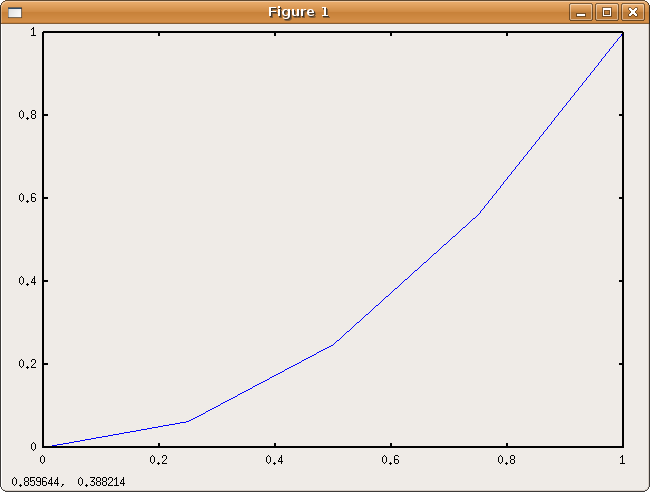
octave:1> x = 0:.25:1 x = 0.00000 0.25000 0.50000 0.75000 1.00000 octave:2> y = x.^2 y = 0.00000 0.06250 0.25000 0.56250 1.00000 octave:3> plot(x,y)
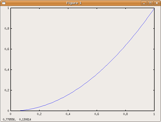
Notice that the plot merely consists of line segments connecting consecutive data points. The plot command makes no attempt to draw a smooth curve between data points. We can however easily produce a smoother looking curve simply by decreasing the spacing between inputs. With the colon operator we can increase our resolution by a factor of 25 just by changing .25 to .01 in the middle. Since we don't really want to see all these numbers displayed in the command window we'll end our input line with a semicolon ; to suppress the textual display of our new 101 x values. Ditto for y.
octave:4> x = 0:.01:1; octave:5> y = x.^2; octave:6> plot(x,y)
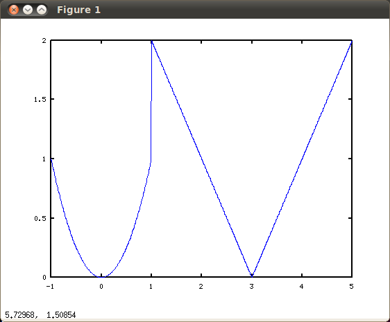
The next example illustrates one of many methods for plotting a piecewise-defined function in Octave or MATLAB. In this example we plot the function $f$ defined by
$\displaystyle{ f(x) = \left\{ \begin{array}{lcl} x^2 & , & x<1 \\ 3-x & , & 1\leq x\leq 3 \\ x-3 & , & x>3 \end{array} \right.} $
over the interval $[-1,5]$.
The input
octave:1> x = -1:.01:5; octave:2> phase1 = x<1; phase2 = (1<=x)&(x<=3); phase3 = x>3; octave:3> y( phase1 ) = x( phase1 ).^2; octave:4> y( phase2 ) = 3 - x( phase2 ); octave:5> y( phase3 ) = x( phase3 ) - 3; octave:6> plot(x,y)
produces
 .
.
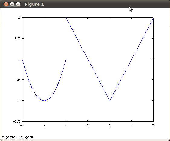
Using the above method, the jump discontinuity at $x=1$ produces a (nearly) vertical segment in the plot. If this is considered undesirable, the following alternative approach may be used. The code below uses the hold on command to combine multiple plots on the same axes in the current figure window.
octave:1> x = -1:.01:1; octave:2> y = x.^2; octave:3> plot(x,y) octave:4> hold on octave:5> x = 1:.01:3; octave:6> y = 3-x; octave:7> plot(x,y) octave:8> x = 3:.01:5; octave:9> y = x-3; octave:10> plot(x,y)
produces
 .
.
Alternative methods for creating arrays (evenly spaced and otherwise) as well as options for the plot command and other plotting routines will be explored in later pages. Also, more useful applications of functions as well as a different approach to working with functions via the Symbolic Toolbox will be introduced.
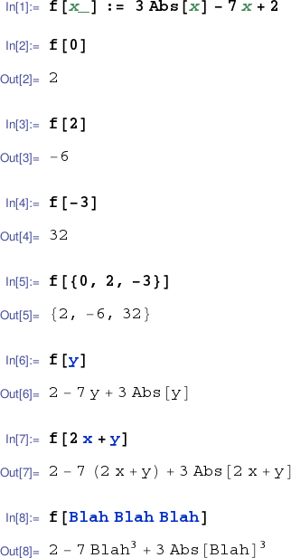
In Mathematica we can implement the function $f$ which
takes each $x$ in $\mathbb{R}$ to $3|x|-7x+2$ with the
definition f[x_] := 3 Abs[x] - 7x + 2.
The underscore is a pattern matching character called Blank.
A Blank matches any expression.
(Note about variable names
in Mathematica.)
After entering the definiton above, invoking
f[expr]
causes Mathematica to (temporarily) give the name
x
to expr,
whatever expr is
(a number, a symbol, a list, whatever).
The right hand side of the definition
(here 3 Abs[x] - 7x + 2)
is then evaluated using the
current meaning of x and returned as output.
Omitting the colon in a function definition is still
syntactically correct, but bears a slightly different
meaning. With :=
(called SetDelayed) the
right hand side is left completely unevaluated at the
time of function definition.
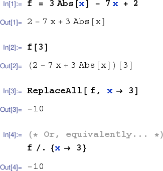
With a bare = (called Set)
the right hand side is evaluated at the time
of function definition. This "preprocessed" form is
then further evaluated at the time of function invocation
according to the pattern matching and substitution process
described above.
The following notebook session illustrates this difference.

The definition f = 3 Abs[x] - 7x + 2 does not define f as a function, but rather as a simple expression. While this distinction is significant, it's still possible to evaluate f for arbitrary values of x using replacement rules. See below.
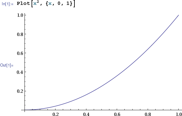
The basic Plot[] command in Mathematica accepts
an expression to be plotted together with an interval over which
the plot is to be constructed. This interval is specified as
a curly-brace delimited, comma separated
list with the input variable given first,
then the lower endpoint of the input interval, and finally the
upper endpoint of the input interval.
In the sample below, the squaring function is plotted over the
interval from 0 to 1. Mathematica is case-sensitive
so plot is not equivalent to
Plot. Note
also that parentheses may not be substituted for square brackets
(for invoking commands) or curly braces (for delimiting lists).
The exponent may be entered from the keyboard using
Ctrl+6 or
by selecting the superscript form from the Basic Math Assistant
Palette. Alternatively x^2 may be used in place of
x2. (Remember to use
Shift-
Enter
to evaluate the cell.)
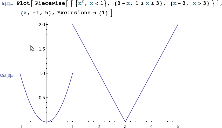
The next example illustrates one way to plot the piecewise-defined function
$\displaystyle{ f(x) = \left\{ \begin{array}{lcl} x^2 & , & x<1 \\ 3-x & , & 1\leq x\leq 3 \\ x-3 & , & x>3 \end{array} \right.} $
over the interval $[-1,5]$ in Mathematica.
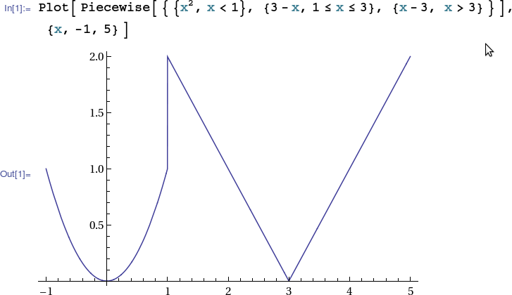
The vertical segment at the jump discontinuity where $x=1$ may be prevented using the Exclusions option.
Options of the Plot[] command as well as other Mathematica plotting routines will be introduced in later pages.
An example of a simple function definition in Sage appears below in the subsection on piecewise functions. But if you're really interested in becoming a Sage guru, take a look at www.sagemath.org/doc/tutorial/tour_functions.html for a discussion of the vagaries of functions and function-like objects in Sage.
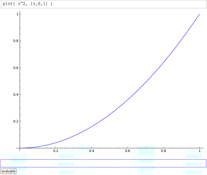
The basic plot() command in Sage accepts an expression to be plotted together with an interval over which the plot is to be constructed. This interval is specified in parentheses with the input variable listed first, then a comma, then the lower endpoint, another comma, and then the upper endpoint. (If the interval specification is omitted, then the default interval from -1 to +1 will be used.) The image below shows a command to plot the squaring function on [0,1] entered in a command box in a Sage Notebook. Note that the thin vertical bar at the right of the input is just a cursor and not part of the input.

And here's what you get after clicking the
![]() button (or, alternatively, typing
Shift-
Enter
within the command box).
button (or, alternatively, typing
Shift-
Enter
within the command box).
Better yet. Give Sage a try by editing the plot() command in the cell below and then clicking the evaluate button. Your command will be sent to a Sage Cell Server which will execute the command for you and return the results to your browser. (Note that this doesn't work seemlessly on all platforms. In particular this doesn't work with some common smart phone browsers with their default configurations. If it does work on your smart phone, but produces a plot which is too wide for your narrow screen, try modifying the input to plot( sin(x) - x^2, (x,0,2), figsize=4 ) and adjusting the figsize option value. )
The piecewise-defined function
$\displaystyle{ f(x) = \left\{ \begin{array}{lcl} x^2 & , & x<1 \\ 3-x & , & 1\leq x\leq 3 \\ x-3 & , & x>3 \end{array} \right.} $
may be plotted in Sage as follows.

Remember that whitespace is significant in (Python-based) Sage, so the example above will not work if proper indentation is not used.

Feel free to scroll back to the editable cell above and attempt to graph a piecewise defined function with Sage. Again, be careful with indentation.
Subsequent pages will introduce options of the plot() command as well as other methods of producing plots in Sage.