
This page introduces methods for computing numerical approximations of definite integrals.
Suppose $x_0,\ldots,x_n$ gives the partition of interval $[a,b]$ into $n$ evenly spaced subintervals, i.e. suppose $x_i = a+i\Delta x$ for $i=0,\ldots,n$ with $\Delta x = \frac{b-a}{n}$. Then if y stores the values of $f$ at $x_0,\ldots,x_n$ in a row vector and h holds the common length of all subintervals (namely $\Delta x=\frac{b-a}{n}$), then h * trapz(y) gives the trapezoidal method approximation to ${\displaystyle \int_a^b f(x)\,dx}$ for the partition $x_0,\ldots,x_n$.
The code below computes the trapezoidal approximations to $\int_0^3 x^2\,dx$ first using the partition with 20 evenly spaced subintervals, then using 100 subintervals.
>> a=0; b=3; n=20; >> h=(b-a)/n; >> x=a:h:b; >> y=x.^2; >> h*trapz(y) ans = 9.0113 >> n=100; >> h=(b-a)/n; >> x=a:h:b; >> y=x.^2; >> h*trapz(y) ans = 9.0004
Not surprisingly using more subintervals yields a result closer to the exact value 9.
If x stores a non-evenly spaced partitition of $[a,b]$, and y holds the corresponding values of $f$, then trapz(x,y) computes the trapezodial approximation to ${\displaystyle \int_a^b f(x)\,dx}$ for the given partition. (This syntax can be used for evenly spaced partitions as well, but it's slightly less efficient than our first approach for that common special case.)
>> x=[0 .05 .1 .3 .32 .4 .55 .7 1 1.3 1.4 1.45 1.6 1.8 1.9 2 2.2 2.3 2.6 2.8 2.91 3]; >> y=x.^2; >> trapz(x,y) ans = 9.0217
It's not difficult to write your own implementation of the trapezoidal method in MATLAB. Feel free to do so as an exercise.
Although (as of this writing) MATLAB does not offer a builtin implementation
of Simpson's rule in its most basic form, you can
download
one from the MATLAB Central file exchange.
The code in
simp.m
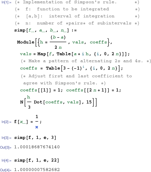
is a barebones implementation of Simpson's rule.
function area = simp( fcn, a, b, n ) % Uses Simpson's rule to approximate the integral of the function % with handle fcn from a to b using n *pairs* of evenly spaced % subintervals. % Author: R Smyth % Version 1.0 8/22/2013 h = (b-a)/(2*n); % Subinterval spacing x = a:h:b; % Partition points y = fcn(x); % Function values at partition points i = 0:2*n; coeffs = 3+(-1).^(i+1); % Kludge to generate pattern of alternating 2s and 4s coeffs(1)=1; coeffs(end)=1; area = h/3 * sum(coeffs.*y); % Simpson's rule formula
octave:1> simp( @(x)x.^2, 0, 3, 1 ) ans = 9 octave:2> format long octave:3> simp( @(x)1./x, 1, exp(1), 3 ) ans = 1.00018687674140 octave:4> simp( @(x)1./x, 1, exp(1), 22 ) ans = 1.00000007582682
Notice that Simpson's rule produced the exact value for $\int_0^3 x^2\,dx$ using just one pair of subintervals. Is this a surprise? Shouldn't be. Simpson's rule uses quadratic approximations and thus produces exact values for quadratic integrands.
MATLAB has several builtin methods for numerically approximating integrals including the integral method (introduced earlier) which uses global adaptive quadrature and the quadgk method (also introduced earlier) which uses adaptive Gauss-Kronrad quadrature. Follow the links to the MATLAB docs for more information about these methods.
Mathematica's numerical integration routine NIntegrate[] (introduced earlier) can be made to use trapezoidal approximations by setting the Method option to "TrapezoidalRule".
If you wish to control the partition you can implement the trapezoidal method as below.
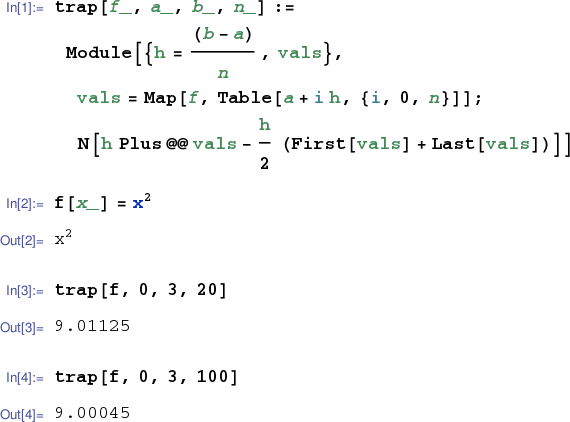
Ordinarily you would use the numerical_integral() command (introduced earlier) to compute numerical approximations to definite integrals in Sage. If you wish to implement the trapezoidal method there are of course many ways to do so, one of which is illustrated below.