This page introduces methods for both exact symbolic computation of definite integrals as well as routines for approximating definite integrals numerically.
The int() command for finding antiderivatives introduced earlier can also compute definite integrals. Just supply the limits of integrations in addition to the integrand.
>> syms x >> int( x^2, 0, 1 ) ans = 1/3 >> int( sqrt(1-x^2), -1, 1 ) ans = pi/2
If your integrand contains a parameter(s) other than the variable of integration you should specify the variable of integration in your call to int() after the integrand and before the limits of integration.
>> syms c x >> int( c*x, x, 0, 1 ) ans = c/2
Some definite integrals have values that cannot be expressed in an elementary form. Others are simply beyond MATLAB's ability to handle. Furthermore there are situations where an exact representation of an integral's value is not helpful. So for a variety of reasons numerical integration is useful. (See the next subsection.)
>> syms x >> int( exp(sin(x)), 0, sym('pi') ) Warning: Explicit integral could not be found. ans = int(exp(sin(x)), x == 0..pi) >> int( sin(x^2), 0, sqrt(sym('pi')) ) ans = (2^(1/2)*pi^(1/2)*fresnelS(2^(1/2)))/2
MATLAB (and Octave) have several methods for numerical integration. We introduce the integral() method through a few simple examples.
>> integral( @(x) x.^2, 0, 1 ) ans = 0.3333 >> integral( @(x) exp(sin(x)), 0, pi ) ans = 6.2088 >> integral( @(x) sin(x.^2), 0, sqrt(pi) ) ans = 0.8948
The integral() method may balk if faced with a highly oscillatory integrand or an integrand which is undefined at an endpoint of integration.
>> integral( @(x) cos(exp(x)), 0, 100 ) Warning: Reached the limit on the maximum number of intervals in use. Approximate bound on error is 1.5e+01. The integral may not exist, or it may be difficult to approximate numerically to the requested accuracy. > In funfun/private/integralCalc>iterateScalarValued at 372 In funfun/private/integralCalc>vadapt at 133 In funfun/private/integralCalc at 76 In integral at 89 ans = -0.602704793970841 >> integral( @(x) sin(1./x), 0, 1 ) Warning: Infinite or Not-a-Number value encountered. > In funfun/private/integralCalc>iterateScalarValued at 349 In funfun/private/integralCalc>vadapt at 133 In funfun/private/integralCalc at 76 In integral at 89 ans = NaN
In some cases these problems can be overcome by tweaking optional arguments to the numerical integrator. (See the docs.) Ironically, these issues can also sometimes be resolved by symbolic computation of the integral (followed by numerical approximation of the result if desired).
>> syms x >> int( cos(exp(x)), 0, 100 ) ans = cosint(exp(100)) - cosint(1) >> vpa( ans, 12 ) ans = -0.337403922901 >> int( sin(1/x), 0, 1 ) ans = sin(1) - cosint(1) >> vpa( ans, 12 ) ans = 0.504067061907
So there are times when you may want an exact symbolic value for a definite integral but are forced to settle for a numerical approximation, while other times you merely need a numerical approximation but find it hard to come by without first performing an exact symbolic computation.
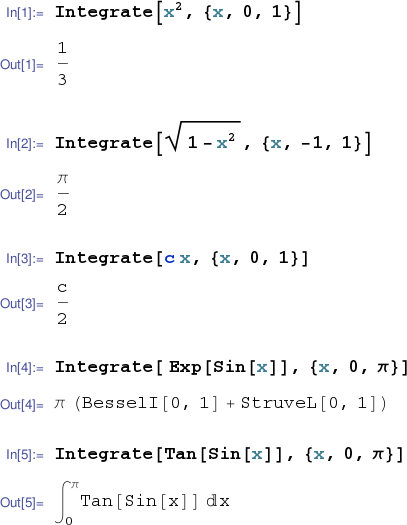
The Integrate[] command introduced in connection with antiderivatives will compute definite integrals if supplied with the limits of integration as in the examples below. Of course it can't handle all possible integrands.
The NIntegrate[] command may be used to compute numerical approximations to definite integrals.
The numerical_integral() command returns both a numerical approximation to a definite integral and a bound on the error in the approximation.