 .
.
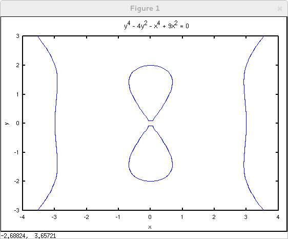
The convenience utility ezplot() may be used to plot implicitly defined functions. First put the equation in the form $f(x,y)=0$. Then pass the expression for $f(x,y)$ to ezplot. Optionally specify a viewing window in the form [xmin xmax ymin ymax]. For example the devil's curve $y^4-4y^2 = x^4-9x^2$ may be plotted in the window $(x,y)\in [-4,4]\times[-3,3]$ with
octave:1> ezplot('y^4 - 4*y^2 - x^4 + 9*x^2', [-4 4 -3 3])
.
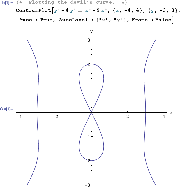
From the perspective of Calc 2, the graph of the function(s) defined implicitly by $f(x,y)=0$ is just the $0$ level curve (or contour) of the two variable function $f$. This perspective leads to an alternative plotting method using the contour() command as illustrated in the Calc 2 TechCompanion page introducing functions of several variables.
Given the simple declaration syms x y the command diff(y,x) will return 0. That is, by default, x and y are treated as independent variables. The declaration syms x y(x), on the other hand, forces MATLAB to treat y as dependent on x facilitating implicit differentiation.
>> syms x y >> diff(y,x) ans = 0 >> syms x y(x) >> diff(y,x) ans(x) = D(y)(x) >> diff( y^4-4*y^2 == x^4-9*x^2, x ) % Implicitly differentiate equation for devil's curve. ans(x) = 4*D(y)(x)*y(x)^3 - 8*D(y)(x)*y(x) == 4*x^3 - 18*x >> pretty(ans(x)) % "Prettyprint" output 3 3 4 D(y)(x) y(x) - 8 D(y)(x) y(x) == 4 x - 18 x
Notice that we were able to pass an equation, rather than a bare expression, to diff(). The equality relation in MATLAB is ==, not to be confused with = which is used for assignment. In the example above it's rather easy now to solve algebraically for ${\displaystyle \frac{dy}{dx}}$ (printed as D(y)(x) in MATLAB) to obtain ${\displaystyle \frac{dy}{dx} = \frac{4x^3-18x}{4y^3-8y}}$. In a messier computation we might wish to let the system do the algebraic step as well as the differentiation. Unfortunately the Symbolic toolbox's algebraic equation solver solve() will not accept D(y)(x) as a symbol to solve for. There is a workaround... but you'll have to wait until you've studied partial derivatives and a more sophisticated version of the chain rule in Calc 2 for the theoretical justification of this workaround! With your equation in the form $f(x,y)=0$, the derivative ${\displaystyle \frac{dy}{dx}}$ of the implicitly defined function is the negative of the quotient of the so-called partial derivatives of $f$ (with the $x$ partial in the numerator and the $y$ partial in the denominator). So in MATLAB, perhaps counter-intuitively, treat x and y as independent, and compute as below.
>> syms x y f >> f = y^4 - 4*y^2 - x^4 + 9*x^2; >> -diff( f, x )/diff( f, y ) ans = (- 4*x^3 + 18*x)/(- 4*y^3 + 8*y) >> pretty(ans) 3 - 4 x + 18 x ------------- 3 - 4 y + 8 y
There are four points on the devil's curve with $x=\frac{1}{2}$. We can compute them exactly with
>> syms x y >> eqn = ( y^4 - 4*y^2 == x^4 - 9*x^2 ); >> % Find points on solution set where x = 1/2. >> eqn1 = subs( eqn, x, 1/2 ) eqn1 = y^4 - 4*y^2 == -35/16 >> solve( eqn1 ) ans = (29^(1/2)/4 + 2)^(1/2) (2 - 29^(1/2)/4)^(1/2) -(29^(1/2)/4 + 2)^(1/2) -(2 - 29^(1/2)/4)^(1/2)
and approximate them with vpa() (variable precision arithmetic).
yvals = vpa( ans, 11 ) yvals = 1.8292870747 0.80852260217 -1.8292870747 -0.80852260217
Using the formula for ${\displaystyle \frac{dy}{dx}}$ obtained above via implicit differentiation we can compute the slopes of the tangents to the curve at the $x=\frac{1}{2}$ points.
>> m = subs( (-4*x^3+18*x)/(-4*y^3+8*y), {x, y}, {[.5;.5;.5;.5], yvals} ) m = -0.86285547867846178823089640632453 1.9522155228223332863008566953148 0.86285547867846178823089640632453 -1.9522155228223332863008566953148
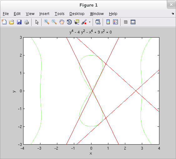
We can now replot the devil's curve together with its tangent lines at the points where $x=\frac{1}{2}$.
>> ezplot('y^4 - 4*y^2 - x^4 + 9*x^2', [-4 4 -3 3]) >> hold on >> x = linspace(-4,4,2); >> y1 = m(1)*(x-.5)+yvals(1); >> y2 = m(2)*(x-.5)+yvals(2); >> y3 = m(3)*(x-.5)+yvals(3); >> y4 = m(4)*(x-.5)+yvals(4); >> plot(x,y1,'r',x,y2,'r',x,y3,'r',x,y4,'r')
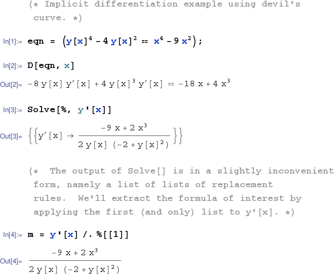
By default Mathematica treats variables as independent. So for example D[y,x] produces 0. Entering y[x] in place of y however tells Mathematica to treat $y$ as a function of $x$. This enables implicit differentiation as in the example below.
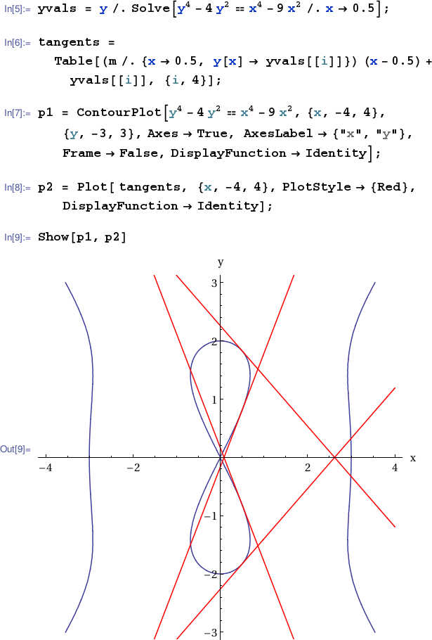
Let's now apply this result to replot the devil's curve together with its tangent lines at the points where $x=\frac{1}{2}$.
Alternatively, using Maxima via Sage...