This page illustrates the syntax for computing limits at infinity as well as the output produced for limits of infinite value in each CAS.
Infinity may be represented by inf or Inf in MATLAB.
>> syms x y >> y = ( 3*abs(x)^3 - 2*x + 1 ) / ( 4*x^3 - x^2 ); >> limit( y, x, inf ) ans = 3/4 >> limit( y, x, -inf ) ans = -3/4
Consider the following examples.
>> syms x y >> y = 1/(x-3)^2; >> limit( y, x, 3 ) ans = Inf >> y = 1/(x-3); >> limit( y, x, 3 ) ans = NaN >> limit( y, x, 3, 'left' ) ans = -Inf >> y = sin(1/x); >> limit( y, x, 0, 'right' ) ans = NaN
All four of the limits considered above, ${\displaystyle \lim_{x\rightarrow 3}\frac{1}{(x-3)^2} }$, ${\displaystyle \lim_{x\rightarrow 3}\frac{1}{x-3} }$, ${\displaystyle \lim_{x\rightarrow 3^-}\frac{1}{x-3} }$ and ${\displaystyle \lim_{x\rightarrow 0^+} \sin{\frac{1}{x}} }$, fail to exist. However, in the first and third examples the manner of divergence may be described as divergence to positive and negative infinity, respectively. In the second and fourth examples the divergence is due to inconsistent behavior to the left and right of the approach point, and undamped oscillation, respectively. In these cases MATLAB simply returns NaN (not a number).
In Octave and MATLAB a polynomial may be represented (without the symbolic toolbox) as an array of coefficients ordered from highest degree to constant term (in a single row). For example, $x^2-3$ may be represented by [1 0 -3]. The deconv() command accepts two polynomials, encoded as above, and performs polynomial division. The invocation syntax is deconv( numerator-polynomial, denominator-polynomial ). By default, only the polynomial quotient is returned. But if the call provides a row array with two variables to store the command's output (as below) then the polynomial quotient is stored in the first variable, and the remainder in the second.
octave:1> num = [1 0 -3]; octave:2> denom = [2 -4]; octave:3> [quot rem] = deconv( num, denom ) quot = 0.50000 1.00000 rem = 0 0 1
The above computation yields ${\displaystyle \frac{x^2-3}{2x-4} = \left(\frac{1}{2}x+1\right) + \frac{1}{2x-4}}$.
Of course the results of polynomial division facilitate identification of dominant terms in rational functions corresponding to certain tendencies of the input.
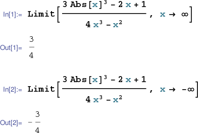
The symbol for infinity may be entered into a Mathematica notebook
with the keyboard sequence
Esc
inf
Esc
and may be used as the approach point in a
Limit[] computation.
Consider the following example computations.
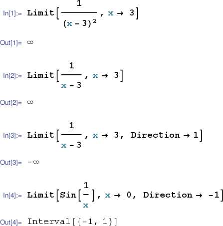
The expression ${\displaystyle \frac{1}{x-3}}$ diverges to $+\infty$ as $x$ approaches $3$ from the right, and to $-\infty$ as $x$ approaches $3$ from the left. Due to this (huge) discrepancy, the divergence of the bidirectional limit at $3$ cannot be described as either divergence to $+\infty$ or divergence to $-\infty$. So it may appear that Mathematica has given an incorrect answer in the second computation above. Note, however, that the Limit[] command in Mathematica does not compute bidirectional (i.e. two-sided) limits. If a direction is not specified, then the default direction (from the right for finite approach points) is used.
In the last example above Mathematica's output not only let's us know that the limit does not exist, but also let's us know that the set of accumulation points of ${\displaystyle \sin{\frac{1}{x}}}$ as $x$ goes to $0$ from the right is the entire interval $[-1,1]$. (This result is suggested by our previous graph.)
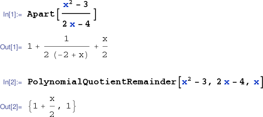
The Apart[] command computes the partial fractions decomposition of a rational function. This decomposition has many uses including identification of dominant terms for certain input tendencies. Alternatively, the PolynomialQuotientRemainder[] command may be used to perform polynomial division.
The approach points $\infty$ and $-\infty$ can be entered in Sage as +Infinity and -Infinity, respectively. (Infinity, without a plus or minus sign, represents complex infinity.)
Sage can perform partial fraction decompositions.
Sage can use a maxima method to perform polynomial division.