On this page we explore the use of numerically generated tables to make educated guesses about limits of functions. Special attention is given to some of the pitfalls of this approach.
Suppose we wish to determine the limit of ${\displaystyle \frac{\sin{2x}-2x}{x^3}}$ as $x$ approaches $0$. We could compute the value of the expression for inputs $x$ that get progressively closer to the approach point $0$ and try to guess what value (if any) these outputs are approaching. The Octave code below computes ${\displaystyle \frac{\sin{2x}-2x}{x^3}}$ for $x = 1$, $0.1$, $0.01$ and $0.001$ and displays the results in a simple table. These results might well inspire a guess that ${\displaystyle \lim_{x\rightarrow 0} \frac{\sin{2x}-2x}{x^3} = \frac{-4}{3}}$. In this case (as in many cases, but certainly not all) the table inspired guess is correct... though a bit tricky to prove without the theory behind Taylor series (usually left until Calc2).
The colon operator used without an increment specification defaults to an increment of 1. So the first input line makes n the array [0 1 2 3 4]. Don't miss the critically important periods in lines 2 and 3. As mentioned earlier the periods give us componentwise operators (as needed here) rather than matrix operators. Line 4 sets the display format. See www.mathworks.com/help/matlab/ref/format.html for details of the format command. The apostrophes in line 5 transpose x and y effectively turning these two rows of numbers into two columns.
octave:1> n = 0:4; octave:2> x = 10.^(-n); octave:3> y = (sin(2*x)-2*x)./x.^3; octave:4> format long g octave:5> [x' y'] ans = 1 -1.09070257317432 0.1 -1.33066920493879 0.01 -1.33330666692022 0.001 -1.33333306678515 0.0001 -1.33333331897058
Now let's try to determine ${\displaystyle \lim_{x\rightarrow 0}\frac{\sqrt{e^x-x-1}}{x}}$.
octave:1> n = 0:4; octave:2> x = 10.^(-n); octave:3> y = sqrt(exp(x)-x-1)./x; octave:4> format long g octave:5> [x' y'] ans = 1 0.847515090401962 0.1 0.71909095917329 0.01 0.708287259294844 0.001 0.707224652069433 0.0001 0.707118570333925
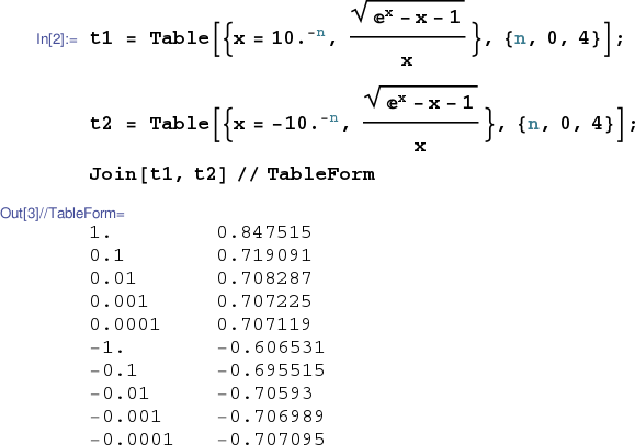
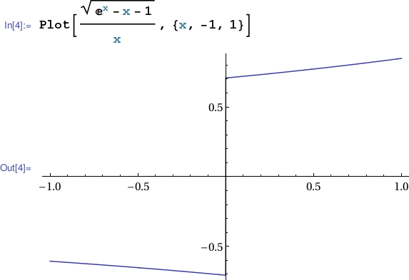
This table might inspire the guess ${\displaystyle \lim_{x\rightarrow 0}\frac{\sqrt{e^x-x-1}}{x}=\frac{\sqrt{2}}{2}}$. In this case, however, ${\displaystyle \frac{\sqrt{e^x-x-1}}{x}}$ has a jump discontinuity at the approach point $0$. While the so-called right-hand limit at $0$ exists and equals ${\displaystyle \frac{\sqrt{2}}{2}}$, the left-hand limit at $0$ has a different value, and so the ordinary or two-sided limit at $0$ does not exist. The moral? At the least we should beef up our procedure by considering inputs from both sides of the approach point, except of course when we only aim to compute a one-sided limit. "Considering" inputs from both sides may involve explicitly including inputs from both sides in our table, or, when appropriate, applying an observed symmetry to deduce behavior on one side from computed behavior on the other. For instance, ${\displaystyle \frac{\sin{2x}-2x}{x^3}}$ is even (at $0$) so its behavior on the left mirrors and matches its behavior on the right, and we lost nothing by including only values to the right of $0$ in our first table. For an odd function computing on both sides is still superfluous. But our conclusion is different. The odd symmetry implies the limit from the left is the negative of the limit from the right. In general, a function which is odd (w.r.t. $a$) either has a two-sided limit of $0$ at $a$, or the limit at $a$ doesn't exist.
Let's re-examine ${\displaystyle \frac{\sqrt{e^x-x-1}}{x}}$ near $x=0$ including inputs from both sides of $0$ in our table.
octave:1> n = 0:4; octave:2> x = 10.^(-n); octave:3> y = sqrt(exp(x)-x-1)./x; octave:4> y = [y sqrt(exp(-x)-(-x)-1)./(-x)]; % Append to y. octave:5> format long g octave:6> [ [x, -x]' y' ] ans = 1 0.847515090401962 0.1 0.71909095917329 0.01 0.708287259294844 0.001 0.707224652069433 0.0001 0.707118570333925 -1 -0.606530659712633 -0.1 -0.695515494864033 -0.01 -0.705930231454324 -0.001 -0.706988949639082 -0.0001 -0.707095003246307
Incidentally, ${\displaystyle \frac{\sqrt{e^x-x-1}}{x}}$ is neither even nor odd, but it's "even part" is relatively insignificant near $0$, and "goes away" in the limit. So the left-hand limit is exactly equal to the negative of the right-hand limit, just like a "pure" odd function.
Another example. Let's examine the behavior of ${\displaystyle \frac{1}{2-x^4-2\cos{x^2}}+\frac{60+2x^4}{5x^8}}$ near $0$. This expression is even, so we'll only use inputs from the right-side of $0$.
octave:1> n = 0:4; octave:2> x = 10.^(-n); octave:3> y = 1./(2-x.^4-2*cos(x.^2)) + (60+2*x.^4)./(5*x.^8); octave:4> format long g octave:5> [x' y'] ans = 1 -0.00623803600442763 0.1 -57.4002785682678 0.01 Inf 0.001 Inf 0.0001 Inf
To make a long story short, the table above is garbage due to the inability of handling such a numerically unstable formula with simple floating point arithmetic. One way to increase the precision of our computations is to use the symbolic toolbox. The syntax for symbolic computations in Octave is not identical to MATLAB's syntax. Since I expect most readers to be using MATLAB rather than Octave, I'll switch to MATLAB for symbolics.
>> syms x y >> y = 1/(2 - x^4 - 2*cos(x^2)) + (60 + 2*x^4)/(5*x^8); >> format long g >> subs(y,x,[1 ; .01 ; .001 ; .0001]) ans = -0.00623803600444236 -0.00619047619095238 -0.00619047619047624 -0.00619047619047619 >> rat( subs(y,x,.0001) ) ans = -0 + 1/(-162 + 1/(2 + 1/(6)))
Notice the declaration of x and y as syms on the first input line, and the absence of componentwise "." operators in the definition of y on line 2. The subs function may be used, as in line 4 above, to replace a symbolic variable by numerical values. This time the computations at least appear stable, and in fact the rat command (cf. www.mathworks.com/help/matlab/ref/rat.html) applied to the last computed value produces the exact value of ${\displaystyle \lim_{x\rightarrow 0} \frac{1}{2-x^4-2\cos{x^2}}+\frac{60+2x^4}{5x^8}}$.
The symbolic toolbox, incidentally, offers a much simpler method for computing the limit under investigation.
>>limit(y,x,0) ans = -13/2100
Of course this command was entered in the same session as above without clearing the definition of y. Obviously the symbolic toolbox limit function is useful for computing limit values, but it's not a panacea for all limit problems. Indeed there are many limits of interest in mathematics whose values are unknown. The symbolic toolbox will be used extensively later in this TechCompanion.
One more example. Let's examine ${\displaystyle \sin{\frac{\pi}{x}}}$ near $0$. (This function is odd, so we'll only perform computations on one side of $0$.)
The table
octave:1> n = 0:4; octave:2> x = 10.^(-n); octave:3> y = sin(pi./x); octave:4> y = [y sin(pi./-x)]; octave:5> format long g octave:6> [ [x, -x]' y' ] ans = 1 1.22464679914735e-16 0.1 -1.22464679914735e-15 0.01 -5.48790321370795e-14 0.001 -7.76163996814028e-13 0.0001 -1.1399618775232e-11 -1 -1.22464679914735e-16 -0.1 1.22464679914735e-15 -0.01 5.48790321370795e-14 -0.001 7.76163996814028e-13 -0.0001 1.1399618775232e-11
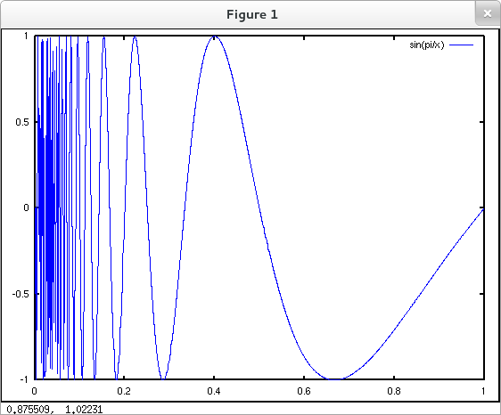
is potentially confusing... but increasing the precision of computation isn't the key here. The value of ${\displaystyle \sin{\frac{\pi}{x}}}$ for $x$ any negative power of $10$ is exactly $0$... but ${\displaystyle \sin{\frac{\pi}{x}}}$ is not going to $0$ as $x$ goes to $0$. Negative powers of $10$ are very special inputs. The value of ${\displaystyle \sin{\frac{\pi}{x}}}$ oscillates between $\pm 1$ ever more wildly as $0$ is approached and so ${\displaystyle \lim_{x\rightarrow 0}\sin{\frac{\pi}{x}}}$ does not exist. (See the rough plot below.)
While the following table is not sufficient to enable a definitive conclusion about the limit, it uses pseudorandom numbers (cf. www.mathworks.com/help/matlab/ref/rand.html) to avoid special inputs and does not create a misleading impression.
octave:1> n = 1:11; octave:2> r = rand(1,11); octave:3> x = (1+r) .* 10.^(-n); octave:4> y = sin(pi./x); octave:5> format long g octave:6> [x' y'] ans = 0.163942862269082 0.308078996989177 0.0135408686447456 -0.452573768207684 0.00108990321614772 -0.999209060137931 0.000111567769723229 -0.487397461244822 1.00533564115395e-05 -0.745274998687196 1.89022312464099e-06 0.228302030578535 1.1827704688101e-07 -0.583752840554757 1.06337234325824e-08 -0.418840549138667 1.50273476374417e-09 0.190480963824975 1.2889005976114e-10 0.687087002448567 1.2556492050312e-11 0.569839895572416
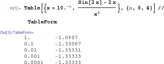
The output of the Table command viewed in TableForm as illustrated below provides a simple and convenient method for viewing a list of input-output pairs for a function of interest. The table below might well inspire the (correct) guess that ${\displaystyle \lim_{x\rightarrow 0}\frac{\sin{2x}-2x}{x^3} = \frac{-4}{3}}$. Notice that the value assigned into x in terms of the iterator n in the first position in the general table entry is available for use in the second position. Notice also that the decimal point after the 10 triggers numerical computation in place of Mathematica's default exact symbolic computation.
The table

only considers values of $x$ to the right of $0$, and thus fails to reveal the jump in ${\displaystyle \frac{\sqrt{e^x-x-1}}{x}}$ at $x=0$. Compare to
or
 .
.
Standard precision arithmetic can produce garbage.
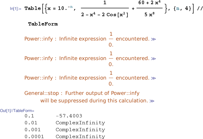
But Mathematica will perform arbitrary precision arithmetic if you ask nicely (say with N[expr,digits-of-precision]). Notice below that the decimal point after the 10 has been removed. This way our nasty expression is first put in an exact symbolic form for each x value, then evaluated with 11 digits of precision as specified. Otherwise standard precision arithmetic would be performed (a game-losing move here) before the N[expr,11] command executes.
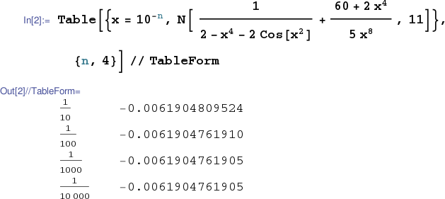
This last table is consistent with
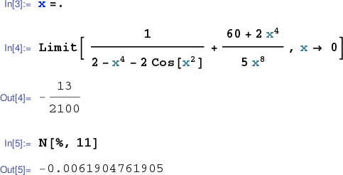 .
.
This last snippet was performed in the same session as the previous computation, which left x with the value $\frac{1}{10000}$. So we first clear x in line 3 with x=., then perform our limit computation. The percentage sign % in Mathematica stands for the result of the previous computation.
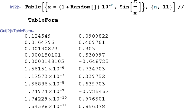
The table
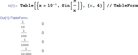
which considers only special input values gives no feel for how $\sin{\frac{\pi}{x}}$ truly behaves close to $x=0$. Introducing some (pseudo)randomness into the input choices gives some hint at the chaos that ensues as $x$ goes to $0$.
Better yet. Take a peek at a plot.

The Sage Cell below illustrates one simple method that may be used in Sage to produce a table of input-output pairs for a function of interest.