Example of motion around a circle (velocity is blue, acceleration is red) mp4 m4v
The following code (prob135no30.m) solves section 13.5 exercise 30 in MATLAB.
% Section 13.5 Problem 30 % R Smyth % Version 1.0: 2/10/2015 syms t r = [ t^3 - 2*t^2 - t, 3*t/sqrt(1+t^2) ]; % Plot the curve. t = linspace(-2,5,222); x = subs(r(1), t); y = subs(r(2), t); plot(x,y) axis equal hold on % Compute v, a, k, T, N. v = diff(r); a = diff(v); k = abs( v(1)*a(2) - v(2)*a(1) ) / norm(v)^3; T = v / norm(v); N = diff(T) / norm(diff(T)); % Determine the center of the osculating circle for the % point where t=1. radius = double(subs( 1/k, 1 )) center = double(subs( r + radius*N, 1 )) % Plot the osculating circle implicitly. [x,y] = meshgrid(-20:.1:5); d = double((x-center(1)).^2 + (y-center(2)).^2); contour(x, y, d, [radius^2 radius^2], 'r'); axis([-20 15 -20 10]) % Make a mark at the point where the osculating circle % is tangent to the curve. plot( subs(r(1),1), subs(r(2),1), '*' )
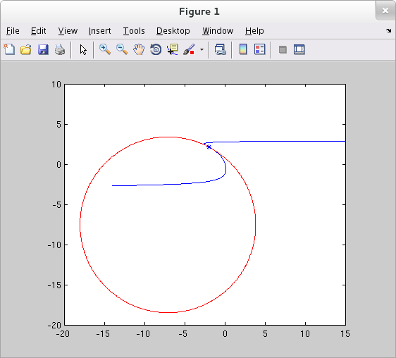
Running the code above produces the following plot.
If you do run this code, I suggest you use the zoom tool to explore how well the osculating circle approximates the curve near the point of tangency.