
The MATLAB function conchoid listed below uses parametric equations for a conchoid to compute the conchoid's second derivative and to plot the conchoid.
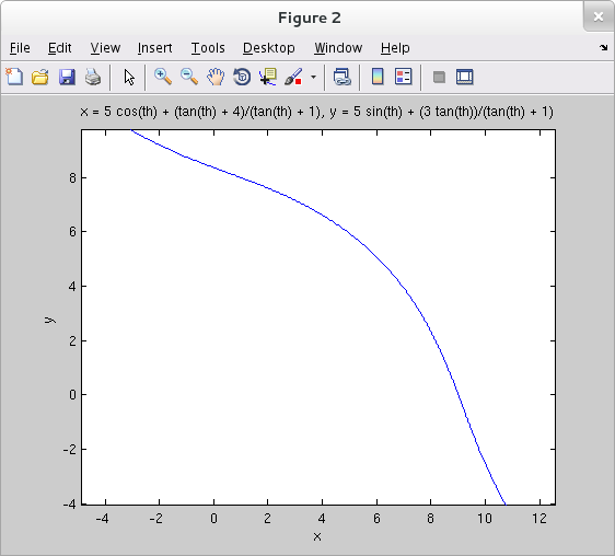
function [xFcn, yFcn, secondDeriv] = conchoid() % Compute the second derivative for example curve presented % in class (as a prelude to finding its inflection points), % and plot the curve. % Return the coordinate functions *and* the second derivative. syms th x = (4 + tan(th)) / (1 + tan(th)) + 5*cos(th); y = 3*tan(th) / (1 + tan(th)) + 5*sin(th); % Compute first derivative. dydx = diff(y,th) / diff(x,th); % Compute second derivative. d2ydx2 = diff(dydx,th) / diff(x,th); % Display the formula for the second derivative. disp(d2ydx2) % Convert coordinate functions and second derivative to % matlab functions... and pass them to the calling % environment. xFcn = matlabFunction(x); yFcn = matlabFunction(y); secondDeriv = matlabFunction(d2ydx2); % Plot the second derivative (as a function of the parameter 'th'). % The zeros of this function give the parameter values % corresponding to the points of inflection on the curve. % These zeros may be approximated from the plot, then % computed precisely with fzero. thVals = linspace(-pi/4+0.01, 3*pi/4-0.01, 111); y1 = zeros([111, 1]); y2 = subs( d2ydx2, th, thVals ); plot( thVals, y1, thVals, y2 ); % Create a new figure window and plot the curve. figure ezplot(x, y, [-pi/8, 5*pi/8])
Executing this function with the command [x, y, d2] = conchoid produces two figures and stores the coordinate functions and the second derivative (as a function of the parameter) into workspace variables x, y, and d2. It always displays the second derivative formula -((5*sin(th) + (6*(tan(th)^2 + 1)^2)/(tan(th) + 1)^2 - (6*tan(th)*(tan(th)^2 + 1))/(tan(th) + 1) + (6*tan(th)^2*(tan(th)^2 + 1))/(tan(th) + 1)^2 - (6*tan(th)*(tan(th)^2 + 1)^2)/(tan(th) + 1)^3)/(5*sin(th) - (tan(th)^2 + 1)/(tan(th) + 1) + ((tan(th) + 4)*(tan(th)^2 + 1))/(tan(th) + 1)^2) + ((5*cos(th) + (3*(tan(th)^2 + 1))/(tan(th) + 1) - (3*tan(th)*(tan(th)^2 + 1))/(tan(th) + 1)^2)*(5*cos(th) + (2*(tan(th)^2 + 1)^2)/(tan(th) + 1)^2 - (2*(tan(th) + 4)*(tan(th)^2 + 1)^2)/(tan(th) + 1)^3 - (2*tan(th)*(tan(th)^2 + 1))/(tan(th) + 1) + (2*tan(th)*(tan(th) + 4)*(tan(th)^2 + 1))/(tan(th) + 1)^2))/(5*sin(th) - (tan(th)^2 + 1)/(tan(th) + 1) + ((tan(th) + 4)*(tan(th)^2 + 1))/(tan(th) + 1)^2)^2)/(5*sin(th) - (tan(th)^2 + 1)/(tan(th) + 1) + ((tan(th) + 4)*(tan(th)^2 + 1))/(tan(th) + 1)^2). (If you weren't already convinced that this problem is best handled with the help of a CAS this formula should sway your opinion.)
From the first plot we see that ${\displaystyle \frac{d^2y}{dx^2}}$ is $0$ for two values of the parameter that are strictly within the parameter's domain, namely the open interval ${\displaystyle (-\frac{\pi}{4},\frac{3\pi}{4})}$. The first of these values is clearly between -0.5 and 0.5, while the second is clearly between 1 and 2. These values can be computed precisely with fzero.
>> th1 = fzero( d2, [-.5, .5]) th1 = -0.0616 >> th2 = fzero( d2, [1, 2]) th2 = 1.6324
The corresponding points on the conchoid may be computed with the coordinate functions.
>> [x(th1) y(th1)] ans = 9.1878 -0.5053 >> [x(th2) y(th2)] ans = 0.4947 8.1878
These points may be marked on our plot of the conchoid as follows.
>> xmarkers = [x(th1) x(th2)]; >> ymarkers = [y(th1) y(th2)]; >> hold on >> plot( xmarkers, ymarkers, 'r*' );
And here's what the result looks like.
