This page takes the subsection on integrals of products of sines and cosines as the inspiration for a terse, informal digression on Fourier sine series.
Notice the prima facie similarity between the operation of dotting two vectors from $\mathbb{R}^n$ and the operation of integrating the product of two (real-valued) functions over an interval. To dot vectors we multiply corresponding components then add the results. When integrating a product, the multiplication is performed pointwise and then the definite integral, in a sense, sums the result. (Technically the integral is a limit of Riemann sums.) Further analysis reveals some critical shared algebraic properties. For instance the property $\int_a^b (c_1 f_1(x) + c_2 f_2(x))g(x)\, dx$ $ = c_1 \int_a^b f_1(x)g(x)\,dx + c_2\int_a^b f_2(x)g(x)\,dx$ mirrors the property $(c_1 \vec{u}_1 + c_2 \vec{u}_2)\cdot \vec{v}$ $ = c_1(\vec{u}_1\cdot\vec{v})+c_2(\vec{u}_2\cdot\vec{v})$. These correspondences inspired a generalization of basic linear algebra to a theory which has proven useful for the analysis of functions.
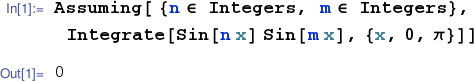
By analogy with basic linear algebra, we can define functions to be orthogonal on an interval if the integral of their product over the interval is $0$. This yields a tantalizing interpretation of the following integration result.
(Note that Mathematica performs simplifications under the assumption that parameters have "generic" values. The result above, in particular, is not valid in the special case $m=n$.) The so-called harmonic frequencies of the sine function on $[0,\pi]$ are orthogonal to each other and to the fundamental frequency. From basic linear algebra we can project $\vec{u}$ onto the line spanned by $\vec{v}$ with the formula ${\displaystyle proj_\vec{v}\vec{u}=\frac{ \vec{u}\cdot\vec{v} }{ \vec{v}\cdot\vec{v} }\vec{v}}$. More generally we can project $\vec{u}$ onto the space $V$ spanned by pairwise orthogonal vectors $\vec{v}_1,\ldots,\vec{v}_k$ with ${\displaystyle proj_V\vec{u}= \sum_{m=1}^k\frac{ \vec{u}\cdot\vec{v}_m }{ \vec{v}_m\cdot\vec{v}_m }\vec{v}_m}$. Analogously we can project the real-valued function $f$ (defined on $[0,\pi]$) onto the function space spanned by the orthogonal set $\{\sin{x},\sin{2x},\ldots,\sin{k x}\}$ with ${\displaystyle proj(f(x))= \sum_{m=1}^k \frac{ \int_0^\pi f(x)\sin{m x}\,dx }{ \int_0^\pi \sin{m x}\sin{m x}\,dx } \sin{m x} }$. This produces a frequency decomposition of $f$. Expanding the set of frequencies that you use, i.e. increasing $k$, expands the space you're projecting onto. This in general makes the projection a better approximation to the original function $f$. (In fact, for a broad class of functions $f$, letting $k$ go to infinity produces a series which converges to $f$ in a certain technical sense. Consider taking Ma401 Boundary Value Problems if you're interested in learning more about this.) Try it out with the Sage interact below.