When integrating a rational function with a CAS there's no need to walk the system through the conventional stages of the computation. In particular, there's no need to explicitly produce the partial fraction representation of the integrand. You can just feed the system your integral and let it produce the final answer without showing you its internal workings or intermediate results. However, the partial fraction decomposition is interesting in its own right and has applications beyond its use in facilitating integration. So this page will look at the commands to use in each target CAS to produce partial fraction representations.
MATLAB does not have a native method for computing partial fraction decompositions with respect to the real numbers $\mathbb{R}$. However the MuPAD function partfrac can be called from the MATLAB command window as in the examples below. By default partfrac produces partial fraction decompositions over the rationals $\mathbb{Q}$. But partfrac will work (approximately) over $\mathbb{R}$ (or $\mathbb{C}$) if the option Domain = R_ (or Domain = C_) is specified.
>> syms x >> feval(symengine,'partfrac', x^7/(x^5 + 4*x^4 + 7*x^3 + 8*x^2 + 5*x + 2), x) ans = ((2*x)/3 + 1/3)/(x^2 + x + 1)^2 - 128/(9*(x + 2)) - 4*x - ((16*x)/9 + 20/9)/(x^2 + x + 1) + x^2 + 9 >> pretty( ans ) 2 x 16 x --- + 1/3 ---- + 20/9 3 128 9 2 ------------- - --------- - 4 x - ----------- + x + 9 2 2 9 (x + 2) 2 (x + x + 1) x + x + 1 >> feval(symengine,'partfrac', 1/((x-1)*(x-2)*(x-3)), x) ans = 1/(2*(x - 1)) - 1/(x - 2) + 1/(2*(x - 3)) >> pretty( ans ) 1 1 1 --------- - ----- + --------- 2 (x - 1) x - 2 2 (x - 3) >> feval(symengine,'partfrac', 1/(x^2-2), x) ans = 1/(x^2 - 2) >> pretty( feval(symengine,'partfrac', 1/(x^2-2), x, 'Domain = R_') ) 0.35355339059327376220042218105242 0.35355339059327376220042218105242 ------------------------------------- - ------------------------------------- x - 1.4142135623730950488016887242097 x + 1.4142135623730950488016887242097
Partial fraction decompositions with respect to the complex numbers $\mathbb{C}$ may be computed with the builtin MATLAB command residue(). The numerator and denominator of the rational function to be decomposed should be passed to residue() as row arrays of coefficients. By default residue() merely returns an array containing the values of the residues at the poles of the given rational function. These residues correspond to numerators in the partial fraction decomposition over $\mathbb{C}$. However if you supply three variables for the output, residue() will also return the locations of the poles and the so-called direct term (if any). The direct term is the polynomial quotient in the case where the degree of the numerator is greater than or equal to the degree of the denominator. A residue of value $r$ occurring at a pole $p$ corresponds to a summand of the form $\frac{r}{(x-p)^m}$ in the partial fractions decomposition. The value of $m$ is $1$ at simple poles, but $m$ "counts up" for repeated poles. See the example below.
>> [r p k] = residue([1 0 0 0 0 0 0 0],[1 4 7 8 5 2]) r = -14.2222 + 0.0000i -0.8889 + 0.7698i -0.0000 - 0.1925i -0.8889 - 0.7698i -0.0000 + 0.1925i p = -2.0000 + 0.0000i -0.5000 + 0.8660i -0.5000 + 0.8660i -0.5000 - 0.8660i -0.5000 - 0.8660i k = 1 -4 9
The input arrays [1 0 0 0 0 0 0 0] and [1 4 7 8 5 2] encode the polynomials $x^7$ and $x^5+4x^4+7x^3+8x^2+5x+2$, respectively. So in effect we're passing residue() the same rational function that we already decomposed with partfrac in the first example on this page. However the earlier result showed that the denominator has $x^2+x+1$ as a factor. Although this quadratic is irreducible over the rationals (and the reals), it can (like any polynomial) be factored into linear terms using complex numbers. Since residue() works over $\mathbb{C}$ not $\mathbb{R}$ or $\mathbb{Q}$, we shouldn't expect exactly the same decomposition as before. The (approximate) residue of $-14.2222$ at the simple pole at $-2$ corresponds to the summand ${\displaystyle \frac{-14.2222}{x-(-2)}}$ in the partial fraction representation. (This matches the term ${\displaystyle -\frac{128}{9(x+2)}}$ from our first crack at this problem... except for rounding in the decimal form.) The (ordered) residues that line up with the second order pole at $-0.5+0.866i$ correspond to two summands in the partial fraction decomposition, namely ${\displaystyle \frac{-0.8889+0.7698i}{x-(-0.5+0.866i)} + \frac{-0.1925i}{(x-(-0.5+0.866i))^2}}$. Similarly the residues at $-0.5-0.866i$ correspond to ${\displaystyle \frac{-0.8889-0.7698i}{x-(-0.5-0.866i)} + \frac{0.1925i}{(x-(-0.5-0.866i))^2}}$. (These last four summands [approximately] match the two summands from the output of partfrac with $x^2+x+1$ in the denominator. Notice that in $\mathbb{C}$ the quadratic $x^2+x+1$ factors into $(x-[\frac{-1}{2}+\frac{\sqrt{3}}{2}i])(x-[\frac{-1}{2}-\frac{\sqrt{3}}{2}i) \approx (x-[-0.5+0.866i])(x-[-0.5-0.866i])$.) The vector k = [1 -4 9] describes the direct term $x^2-4x+9$. This matches the polynomial part returned by partfrac.
The second illustration of partfrac above used a rational function whose denominator did not contain any quadratics that are irreducible over $\mathbb{Q}$. So in this case residue() should produce the same answer, just in a different format. And so it does.
>> syms x >> expand( (x-1)*(x-2)*(x-3) ) ans = x^3 - 6*x^2 + 11*x - 6 >> [r p k] = residue([1],[1 -6 11 -6]) r = 0.5000 -1.0000 0.5000 p = 3.0000 2.0000 1.0000 k = []
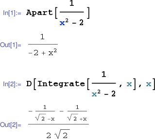
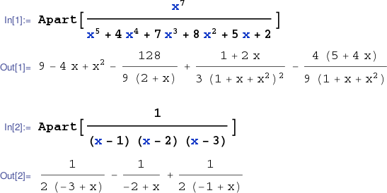
The Mathematica command Apart[] computes partial fraction decompositions over the rationals.
Often the easiest way to compute partial fraction decompositions over the reals in Mathematica is to exploit the Integrate[] command as below. (Unfortunately this little trick does not always produce the desired result.)