Note especially the use of the sum() command (which
sums the elements of a row vector) in
the function estimateArea()
(estimateArea.m).
function areaEstimations = estimateArea( fcn, a, b, n ) % Provides three estimates of the area under the graph of fcn % above the interval [a,b] using n equal width rectangles. % The heights of the approximating rectangles for the three % estimations are computed using fcn values at % left endpoints, midpoints and right endpoints % of the rectangle bases. % If n is an array, then the three estimates are produced for % each n value. % Initialize output array areaEstimations = []; for i=1:length(n) dx = (b-a)/n(i); % Width of each rectangle xl = a:dx:b-dx; % Left endpoints xr = a+dx:dx:b; % Right endpoints xm = (xl+xr)/2; % Midpoints % Add a row with 3 area estimates for each n value. areaEstimations = [ areaEstimations ; dx*[sum(fcn(xl)) sum(fcn(xm)) sum(fcn(xr))] ]; end
Two sample invocations.
octave:1> estimateArea( @(x)1-x.^2, 0, 1, 4 ) ans = 0.78125 0.67188 0.53125 octave:2> estimateArea( @(x)1-x.^2, 0, 1, [2 4 16 50 100 1000] ) ans = 0.87500 0.68750 0.37500 0.78125 0.67188 0.53125 0.69727 0.66699 0.63477 0.67660 0.66670 0.65660 0.67165 0.66667 0.66165 0.66717 0.66667 0.66617
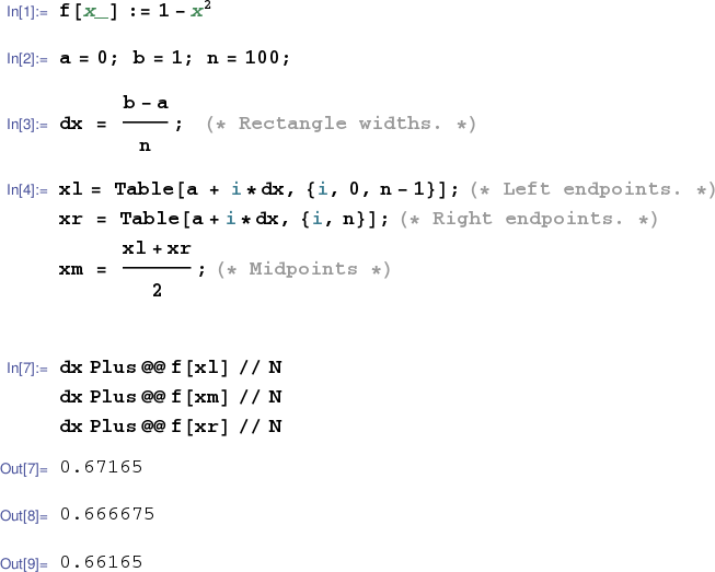
The Mathematica notebook session belows illustrates the use of Mathematica to compute sums of the form $f(c_1)\Delta x + f(c_2)\Delta x + \cdots + f(c_n)\Delta x$ which arise when estimating the area under a portion of the graph of $f$ using rectangles.