This page considers exercise 4.5 #68.
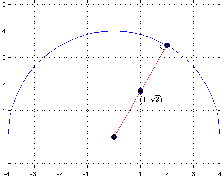
(a) How close does the semicircle $y=\sqrt{16-x^2}$ come to the point $(1,\sqrt{3})$?
Let's first approach this question without using calculus. Let $P=(1,\sqrt{3})$ and let $Q$ be the point of the semicircle closest to $P$. The segment $\overline{PQ}$ must be perpendicular to the semicircle at $Q$. It follows that $\overline{PQ}$ lies along a radius of the semicircle. The radius of the semicircle which passes through $P$ has equation $y-0=\frac{\sqrt{3}-0}{1-0}(x-0)$, or $y=\sqrt{3}x$. Substituting into the equation of the semicircle and squaring both sides yields $3x^2=16-x^2$. Of the two solutions of this equation $x=\pm 2$, clearly $x=-2$ is extraneous here. So point $Q$ is $(2,\sqrt{16-2^2})=(2,2\sqrt{3})$, and the distance from $P$ to the semicircle is $\sqrt{(2-1)^2 + (2\sqrt{3}-\sqrt{3})^2}=2$.
The illustration above was created in MATLAB with the script in file ex_4_5_68aGraphic.m.
% ex_4_5_68aGraphic.m % Script file to create graphic for Prob. 4.5 #68a. % plot semicircle x = linspace(-4,4,100); y = sqrt(16-x.^2); plot(x,y); hold on; grid on; axis equal; % force correct aspect ratio % plot origin, point (1,sqrt(3)), and closest point on semicircle plot([0 1 2],[0 sqrt(3) 2*sqrt(3)],'o','MarkerFaceColor','k','MarkerSize',8); % plot radius through (1,sqrt(3)) plot([0 2],[0 2*sqrt(3)], 'color', 'red'); % annotate (1,sqrt(3))... use LaTeX to get a nice radical sign text(1, sqrt(3)-.3, '$(1,\sqrt{3})$', 'Interpreter', 'Latex', 'FontSize', 12); % add right angle marker ep = .1; plot(2+[-ep -ep*(1+sqrt(3)) -ep*sqrt(3)], 2*sqrt(3)+[-ep*sqrt(3) ep*(1-sqrt(3)) ep], 'k'); h = gcf; % get a handle to the current figure set(h, 'color', 'w'); % change background color of figure to white
Alternatively we can use standard calculus techniques to minimize $f(x) = dist( (1,\sqrt{3}), (x,\sqrt{16-x^2}) ) = \sqrt{(x-1)^2 + (\sqrt{16-x^2}-\sqrt{3})^2}$ over the interval $[-4,4]$. To simplify our work notice that the $x$ value which minimizes $f(x)$ will also minimize the simpler function $g(x)=(f(x))^2=x^2-2x+1+16-x^2+3-2\sqrt{3}\sqrt{16-x^2}=20-2x-2\sqrt{3}\sqrt{16-x^2}$. The derivative $g'(x)=-2-2\sqrt{3}\frac{1}{2}(16-x^2)^\frac{-1}{2}(-2x)=\frac{-2\sqrt{16-x^2}+2\sqrt{3}x}{\sqrt{16-x^2}}$ exists everywhere on the open interval $(-4,4)$ and is zero iff the numerator is zero. So $g'(x)=0$ when $2\sqrt{16-x^2}=2\sqrt{3}x$. Dividing by $2$ then squaring both sides yields $16-x^2=3x^2$ which implies $x=\pm 2$. From the equation before we squared both sides (or the original problem) we can see that $x=-2$ is extraneous. Since $g'$ is continuous on $(-4,2)$ and doesn't have any zeros there, it must maintain the same sign over the whole interval. Plugging in a sample value from the interval, say $x=0$, reveals that this sign is negative. Similar reasoning reveals that $g'$ is positive everywhere on the open interval $(2,4)$. According to the First Derivative Test for Local Extrema the transition in the sign of $g'$ from negative to positive at $x=2$ reveals that $g$ has a local min at $x=2$. Notice though that $g'$ is negative everywhere on $(-4,2)$ and positive everywhere on $(2,4)$. So $g$ itself is decreasing on $(-4,2)$ and increasing on $(2,4)$. This together with the continuity of $g$ on $[-4,4]$ implies that the local min at $x=2$ is in fact the global min over the interval $[-4,4]$. (Alternatively we could argue that the continuous function $g$ must have a global min on the closed and bounded interval $[-4,4]$, and that the only candidates for where the global min occurs are the endpoints and points where $g'$ equals zero or doesn't exist. This leaves us with only three points to consider, namely $\pm 4$ and $2$. Plugging these three points into $g$ reveals that the global min occurs at $2$.) Now although $x=2$ simultaneously minimizes $g$ and $f$, the minimum values of these two functions aren't the same. Though $g$ was convenient to work with, it's the minimum of $f$ that we really care about. So plug $2$ into $f$ to see that the distance from $(1,\sqrt{3})$ to the semicircle $y=\sqrt{16-x^2}$ is $\sqrt{(2-1)^2+(\sqrt{16-2^2}-\sqrt{3})^2} = \sqrt{1+12+3-2\sqrt{12}\sqrt{3}}=2$.
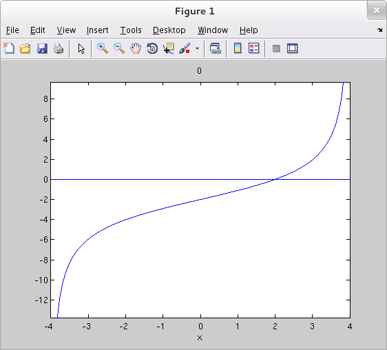
Of course some of this work could be done in MATLAB.
>> syms x f g >> f = sqrt( (x-1)^2 + (sqrt(16-x^2)-sqrt(3))^2 ); >> g = f^2; >> gp = diff(g) gp = 2*x + (2*x*(3^(1/2) - (16 - x^2)^(1/2)))/(16 - x^2)^(1/2) - 2 >> solve( gp==0 ) ans = 2.0 >> ezplot( gp, [-4 4] ) >> hold on >> ezplot( '0', [-4 4] ) % make it easier to see where graph of gp=g' crosses x-axis
(b) Graph the distance function and $y=\sqrt{16-x^2}$ together and reconcile what you see with your answer in part (a).
>> syms x y f >> y = sqrt(16-x^2); >> f = sqrt( (x-1)^2 + (sqrt(16-x^2)-sqrt(3))^2 ); >> ezplot( y, [-4 4] ) >> hold on >> ezplot( f, [-4 4] ) >> axis equal >> line( [-4 2], [2 2], 'LineStyle', '--', 'color', 'k' ) >> line( [2 2], [0 2], 'LineStyle', '--', 'color', 'k' )
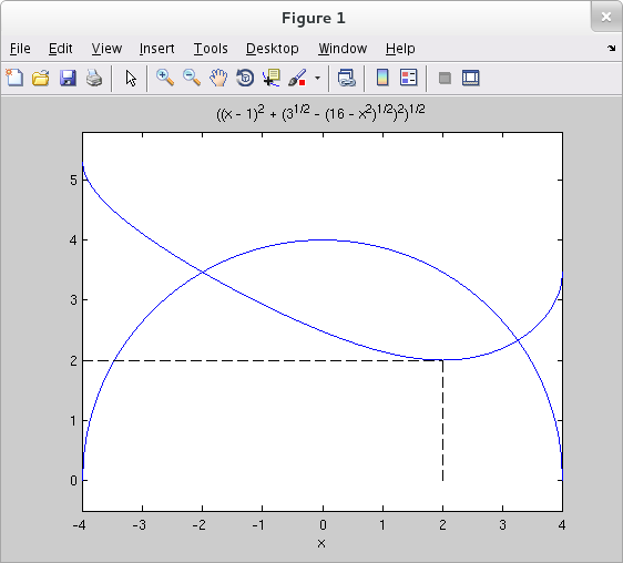
This plot confirms both that the distance is minimized when $x=2$ and that the minimum distance is $2$.