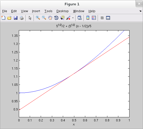
The linearization of $f(x)$ at $x=a$ is one of $f$'s Taylor polynomials at $a$. The Symbolic Toolbox command taylor() may be used to find the linearization of a one variable expression by setting the 'ExpansionPoint' option to the input value at which the linearization is to be based and setting the 'Order' option to 2. In the example below, we plot $\sqrt{x^2+1}$ together with its linearization at $x=0.5$ over the interval $[0,1]$.
>> ezplot( sqrt(x^2+1), [0 1] ) >> hold on >> h = ezplot( taylor( sqrt(x^2+1), 'ExpansionPoint', 0.5, 'Order', 2 ), [0 1] ); >> set(h, 'Color', 'r')
Notice, incidentally, that we stored the handle to the plot of the linearization in h and used this handle to change the color of the line.
See the Calc 2 TechCompanion page on Taylor polynomials for more information about Taylor polynomials in general.
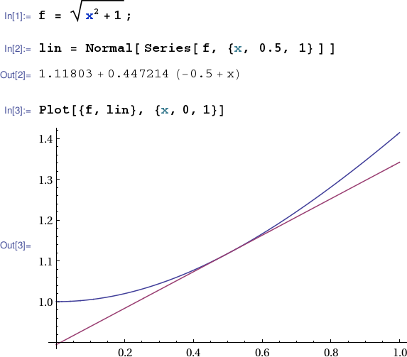
Linearizations can be computed in Mathematica using the syntax Normal[ Series[ expression, {variable, basepoint, 1} ] ]. For example, the notebook session below computes the linearization of $f(x)=\sqrt{x^2+1}$ at $x=\frac{1}{2}$ and plots it together with $f(x)$ over the interval $[0,1]$.