The Octave/MATLAB section of this page introduces a simplistic numerical technique for computing derivatives. Some useful array indexing tricks as well as a method to load data from a file are introduced in the process. The Sage section offers a solution to Exercise 3.2 #62 in the form of a Sage interact.
Suppose for some ascending sequence of values $x_1 < x_2< \cdots < x_n$ in the domain of function $f$ we have the values of the corresponding outputs $y_1=f(x_1)$, $y_2=f(x_2)$,$\ldots$,$y_n=f(x_n)$. If consecutive $x$-values $x_i$, $x_{i+1}$ are sufficiently close, we can construe the secant line through $(x_i, f(x_i))$ and $(x_{i+1},f(x_{i+1}))$ as an approximation to the tangent line through the graph of $f$ at $(x_i, f(x_i))$. So we can approximate $f'(x_i)$ by ${\displaystyle \frac{ f(x_{i+1}) - f(x_i) }{x_{i+1}-x_i} }$. Using this approximation for $i=1,\ldots,n-1$ yields a sequence of points that can be plotted to approximate the graph of $f'$. This (admittedly simplistic) method of numerical differentiation can be readily implemented in Octave (or MATLAB) using the diff() function. If diff() is fed a length $n$ row vector [ $a_1$ $a_2$ $a_3$ $\cdots$ $a_{n-1}$ $a_n$ ] it returns the length $n-1$ row vector of consecutive differences [ $a_2-a_1$ $a_3-a_2$ $\cdots$ $a_n-a_{n-1}$ ]. So if x = [ $x_1$ $x_2$ $x_3$ $\cdots$ $x_{n-1}$ $x_n$ ] and y = [ $y_1$ $y_2$ $y_3$ $\cdots$ $y_{n-1}$ $y_n$ ] = [ $f(x_1)$ $f(x_2)$ $f(x_3)$ $\cdots$ $f(x_{n-1})$ $f(x_n)$ ], then the pointwise quotient diff(y) over diff(x) will yield a row vector of slopes that approximate $f'$ at $x_1,\ldots,x_{n-1}$.
In the example below, we use the
load() command to copy
an array of $x$,$y$ pairs for some "mystery function"
from file
mysteryFunc.dat
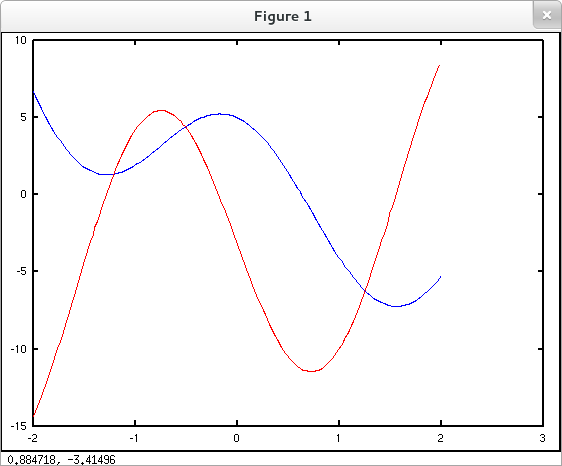
into Octave's workspace. We then implement the method
described above to plot the mystery function and
an approximation to its derivative together.
octave:1> load('mysteryFunc.dat') % Use full pathname if data file is not stored in Octave's working directory octave:2> who % See what variable(s) have been loaded into current workspace Variables in the current scope: ans fncData octave:3> size( fncData ) ans = 2 200 octave:4> % fncData has 2 rows with 200 values each octave:4> % The first row contains x values, octave:4> % and the second row corresponding y values. octave:4> x = fncData(1,:); % Copy the first row into x. octave:5> y = fncData(2,:); % And the second row into y. octave:6> yp = diff(y)./diff(x); % Compute difference quotients. octave:7> plot( x, y, 'b', x(1:end-1), yp, 'r' ) % Plot mystery function and approximation to derivative together.
The data in variable
fncData was created in a previous session
and stored in the file mysteryFunc.dat
with the command
save('mysteryFunc.dat', 'fncData').
(See
www.mathworks.com/help/matlab/ref/save.html
and
www.mathworks.com/help/matlab/ref/load.html
for more information about the
save()
and
load()
commands.)
Note the syntax x(1:end-1) used to create a row vector with all but the last value from row vector x. Perhaps it's worth mentioning that the difference quotient ${\displaystyle \frac{f(x_{i+1})-f(x_i)}{x_{i+1}-x_i}}$ could just as well be construed as an approximation to $f'(x_{i+1})$. We could adapt our code above to this alternative perspective simply by changing x(1:end-1) to x(2:end). Is there any reason to expect a tendency for ${\displaystyle \frac{f(x_{i+1})-f(x_i)}{x_{i+1}-x_i}}$ to approximate $f'$ at the midpoint of $x_i$ and $x_{i+1}$ more accurately than it approximates either $f'(x_i)$ or $f'(x_{i+1})$? How would you adapt the code above to reflect such an alternative approximation scheme?
Under what conditions might the procedure above produce poor results, or even just plain garbage? Clearly if our data points aren't spaced closely enough to reflect the behavior of $f$ accurately we can't expect this method (or any method) to derive an accurate representation of $f'$. See, for instance, the plots below.
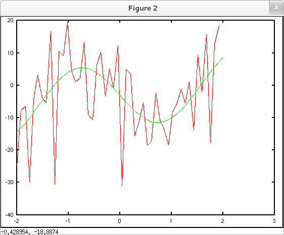
The circles in the plot immediately below represent a poor sampling of the given function. The consecutive difference quotients for this poor sampling are graphed in red in the following plot next to an accurate representation (in green) of the derivative of the original function.
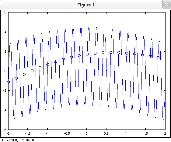
Now suppose that our data points have adequately small (horizontal) spacing, but include inaccuracies in function values. (This is typical of measured values as opposed to values computed from a numerically stable formula.) While in this case a scatter plot of the data may produce a reasonably accurate impression of the underlying function's behavior, our difference quotients may wildly misrepresent the function's derivative. See the plots below.
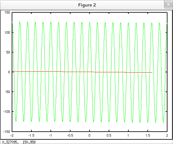
The blue circles represent a "noisy" sampling of the blue curve. The following plot compares the consecutive difference quotients (in red) of the noisy data to an accurate representation (in green) of the derivative of the original underlying function.

Incidentally, scatter plots can be created in Octave and MATLAB with the scatter() command. The syntax for this command is similar to the syntax for the basic plot() command. See www.mathworks.com/help/matlab/ref/scatter.html for details.
The Weierstrass function ${\displaystyle f(x) = \sum_{n=0}^\infty \left(\frac{2}{3}\right)^n\cos{(9^n \pi x)}}$ is continuous everywhere but differentiable nowhere on the real line. Although any partial sum ${\displaystyle g_N(x) = \cos{(\pi x)} + \left(\frac{2}{3}\right)^1\cos{(9\pi x)}+\cdots +\left(\frac{2}{3}\right)^N\cos{(9^N\pi x)}}$ is differentiable (everywhere), zooming in on the graphs of partial sums reveals a dramatic increase in "wiggliness" and "bumpiness" as $N$ increases and the partial sum better approximates the Weierstrass function.
The interact below allows you to select the order of the partial sum and a zoom level with sliders. Regardless of zoom level, the left hand plot will display the partial sum you selected plotted on the interval $[-1,1]$. The right hand plot will response to your zoom selection. The red boxes indicate the portion of the fixed scale plot you've zoomed in on. (Notice that zooming in this tool is not designed to preserve the aspect ratio of the original plot.)
The next interact also allows you to choose the order of a partial sum. Your chosen partial sum and its derivative are plotted side-by-side. Notice how dramatically the maximum value of the derivative increases as the order of the partial sum is increased.