The most common way to represent a real-valued function of a real variable visually is of course to plot a graph of input-output pairs in a coordinate grid formed by a pair of perpendicular input and output axes. The derivative of a function at a particular input point (if it exists) is the slope of the function's graph at the point corresponding to the given input.
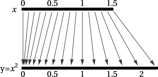
One alternative is to construct parallel input and output axes, treat these axes as screens and treat the function as a lens which effects a projection from the input axis to the output axis. The image below represents the squaring function on $[0,\frac{3}{2}]$ using this alternative paradigm.
The difference quotient ${\displaystyle \frac{f(x+\Delta x)-f(x)}{\Delta x} = \frac{\Delta y}{\Delta x}}$ can now be interpreted as the magnification factor of function $f$ for the interval $[x, x+\Delta x]$. And the derivative ${\displaystyle f'(x)=\lim_{\Delta x\rightarrow 0} \frac{f(x+\Delta x)-f(x)}{\Delta x} = \lim_{\Delta x\rightarrow 0} \frac{\Delta y}{\Delta x}}$ can be interpreted as the magnification factor of $f$ at $x$.
The composite function $f\circ g$ may be applied to the interval $[x, x+\Delta x]$ as a pair of projections in series. First apply $g$ to $[x, x+\Delta x]$ to obtain $[g(x), g(x+\Delta x)]$. For convenience we'll define $u$ as $g(x)$ and $\Delta u$ as $g(x+\Delta x)-g(x)$, so $g$ takes $[x, x+\Delta x]$ to $[u, u+\Delta u]$. Then apply $f$ to $[u, u+\Delta u]$ to obtain $[f(u), f(u+\Delta u)]$, which becomes $[y, y+\Delta y]$ with the appropriate definitions. Apparently the magnificaton factor of $f\circ g$ on $[x,x+\Delta x]$ is the product of the magnification factors of $g$ and $f$ on the intervals $[x,x+\Delta x]$ and $[u,u+\Delta u]$, respectively. (Notice that the magnification factor of $f$ on the original interval $[x,x+\Delta x]$ is irrelevant. In general, $f$ doesn't "see" this interval. It acts on the intermediate interval $[u,u+\Delta u]$.) Intuitively, letting $\Delta x$ go to $0$ forces $\Delta u$ to $0$ and the relationship among magnification factors on intervals yields the following relationship for magnification factors at points. Namely the magnification factor of $f\circ g$ at $x$ is the product of the magnification factors of $g$ and $f$ at $x$ and $u$, respectively. In other words, $(f\circ g)'(x)= g'(x)f'(u) = f'(g(x))g'(x)$. This is the (one-variable) chain rule. (Note that the magnification factor of $f$ at $x$, i.e. $f'(x)$, is irrelevant here.)
If you don't see the technical flaw in our heuristic proof of the chain rule hunt for it in your textbook. In any case, this heuristic, though not rigorous, captures the essence of the one-variable chain rule.
The Sage interact below illustrates our heuristic proof of the chain rule with $g(x)=\sqrt{x}+3$, ${\displaystyle f(u)=\frac{27}{26-4u}}$ and "base point" $x=4$. You can vary $\Delta x$ with a slider. Notice that as $\Delta x$ becomes small the "magnification factor" ${\displaystyle \frac{\Delta u}{\Delta x}}$ approaches ${\displaystyle g'(4)=\left.\frac{du}{dx}\right|_{x=4}=\frac{1}{4}}$, the "magnification factor" ${\displaystyle \frac{\Delta y}{\Delta u}}$ approaches ${\displaystyle f'(g(4))=f'(5)=\left.\frac{dy}{du}\right|_{u=5}=3}$, and the "magnification factor" ${\displaystyle \frac{\Delta y}{\Delta x}}$ approaches ${\displaystyle (f\circ g)'(4)= f'(g(4))g'(4)=f'(5)g'(4)= (\left.\frac{dy}{du}\right|_{u=g(4)=5})(\left.\frac{du}{dx}\right|_{x=4})= \frac{3}{4}}$.