In this section, we advance our understanding of the use of functions in CASs via examples related to average rates of change.
Consider an object in free fall whose distance fallen $y$ (in feet)
after $t$ seconds is approximated by $16t^2$ consistent with Galileo's law.
The average speed of the object over the time interval from time
$t=t_0$ to time $t=t_0+h$ (in ft/s) is, according to this simple model,
${\displaystyle \frac{\Delta y}{\Delta t} = \frac{ 16(t_0+h)^2 - 16t^2 }{ h }}$.
The M-file
avgSpeed.m contains
a function
avgSpeed which accepts numerical values for $t_0$ and $h$
as input, and returns the corresponding average speed.
You can either create your own version of this function in a text
editor or download mine from the link above. Either way pay attention
to the function's syntax and make sure you save the M-file in a
directory on Octave's (or MATLAB's) search path.
Then, at the command prompt, test the function.
octave:1> avgSpeed(1,1) ans = 48
Let's now investigate how this average speed behaves as the length of the time interval is made smaller and smaller by calling avgSpeed from within a for loop that iterates over several h values. (Notice the change in command prompt for this multi-line loop. Execution commences after entering the end keyword. Note also that there really wasn't any need to use the same letter h for the iterator in the command window as is used in the code for function avgSpeed. In general, you shouldn't need to know any details of a function's implementation to use the function.)
octave:2> for h = [1 0.1 0.01 0.001 0.0001] > avgSpeed(1,h) > end ans = 48 ans = 33.600 ans = 32.160 ans = 32.016 ans = 32.002
Alternatively,
octave:3> avgSpeed([1 1 1 1 1], [1 .1 .01 .001 .0001]) ans = 48.000 33.600 32.160 32.016 32.002.
Better yet. Try the script avgSpeedTable to create a formatted table of average speeds.
octave:4> avgSpeedTable Length of Average speed Average speed interval h over [1, 1+h] over [2, 2+h] 1.00000 48.00000 80.00000 0.10000 33.60000 65.60000 0.01000 32.16000 64.16000 0.00100 32.01600 64.01600 0.00010 32.00160 64.00160 0.00001 32.00016 64.00016
The function avgSpeed computes average rates of
change for one specific function. If we wish to compute average
rates of change for some other functions we can of course
create adapted versions of our code for each function of interest.
But a much more elegant and versatile solution is to write code
that let's the user pick the function "on the fly."
This can be achieved using function handles.
The M-file
avgRateOfChange.m
contains the code for an (Octave) function that accepts
a function handle for a (mathematical) function $f$ as well as numerical values
for $x_1$ and $h$, and returns the value of
${\displaystyle \frac{ f(x_1+h) - f(x_1) }{ h } }$.
octave:1> avgRateOfChange( @(t)(16*t^2), 1, 0.1 ) % Equivalent to avgSpeed( 1, 0.1 ) ans = 33.600 octave:2> avgRateOfChange( @(x) sin(x), 0, pi/2 ) ans = 0.63662 octave:3> avgRateOfChange( sin(x), 0, pi/2 ) % Improper call. sin(x) isn't a function handle error: `x' undefined near line 4 column 22 error: evaluating argument list element number 1 error: evaluating argument list element number 1 octave:4> avgRateOfChange( @(x) sin(x), 0, 0 ) % Illegal value for interval length error: Can't compute average rate of change over an empty interval. error: called from: error: /var/www/TechCompanion/Calc1/Ch02/Octave/avgRateOfChange.m at line 10, column 2 octave:5> avgRateOfChange( @(x) (3*x.^2 - 2*sin(x) + 1) , [0 0 0], [pi/2 pi/20 pi/200] ) ans = 3.4391 -1.5205 -1.9528
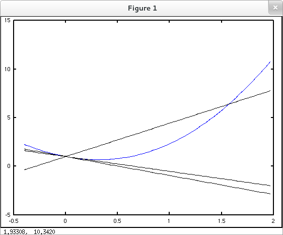
The last computation above gives the average rates of change of the function $f$ given by $f(x) = 3x^2 - 2\sin{x} + 1$ over the intervals $[0,\frac{\pi}{2}]$, $[0,\frac{\pi}{20}]$ and $[0,\frac{\pi}{200}]$, respectively. These average rates of change equal the slopes of the corresponding secant lines on the graph of $f$. Let's construct a plot to accompany our numerical computations. The utility secantLine which generates function handles for secant lines will facilitate our plot construction.
octave:1> f = @(x) 3*x.^2 - 2*sin(x) + 1; octave:2> sec1 = secantLine( f, 0, pi/2 ); octave:3> sec2 = secantLine( f, 0, pi/20 ); octave:4> sec3 = secantLine( f, 0, pi/200 ); octave:5> x = linspace( -.4, pi/2+.4, 100 ); octave:6> y0 = f(x); y1 = sec1(x); y2 = sec2(x); y3 = sec3(x); octave:7> plot( x, y0, 'b', x, y1, 'k', x, y2, 'k', x, y3, 'k' );
Notice that you need to pay attention to the scales on the axes in this plot if you want to approximate the slopes of the secants graphically and compare with the values computed numerically above.