The assertion ${\displaystyle \lim_{x\rightarrow x_0}f(x)=L}$ means that for any positive $\varepsilon$ there exists a positive $\delta$ such that $|f(x)-L|<\varepsilon$ whenever $0<|x-x_0|<\delta$. Symbolically, ${\displaystyle \lim_{x\rightarrow x_0}f(x)=L}$ means ${\displaystyle \forall\varepsilon>0\,\,\exists\delta>0: \forall x \,(0<|x-x_0|<\delta \implies |f(x)-L|<\varepsilon)}$. This precise definition of limit, together with virtually any technical statement involving nested quantifiers, proves to be difficult to master for many students. You may need to reread this definition many times and/or work through extended explanations and alternative perspectives (as given below) before the concept comes into focus for you.
A sloppy, imprecise (but commonly used) description of limits goes as follows. The statement ${\displaystyle \lim_{x\rightarrow x_0}f(x)=L}$ means that $f(x)$ gets close to $L$ when $x$ gets close to $x_0$. (Note that the tabular method for guessing limits from the previous section can readily be abused in a way that reinforces a comparable imprecise conception of limits.) One key problem with the statement above is that we really don't know in general what "close to" means. Guided by the precise formulation we could construct an improved verbalization of the definition of limit as follows. The limit of $f(x)$ as $x$ goes to $x_0$ equals $L$ means that the limit value ($L$) approximates the function output ($f(x)$) to within any prespecified tolerance ($\varepsilon$) at least whenever the inputs ($x$) are restricted to be sufficiently close (within $\delta$ units) of the approach point ($x_0$) without including the approach point exactly.
Now let's try to break this definition down into
more readily digestable chunks.
A choice of a particular value for the "tolerance"
$\varepsilon$
may be construed as a challenge to the limit assertion.
A value for $\delta$ chosen in response to an $\varepsilon$
challenge should be considered an adequate response if
in fact $0<|x-x_0|<\delta \implies |f(x)-L|<\varepsilon$
for the $\varepsilon$-$\delta$ challenge-response pair.
That is to say, the response is adequate if inputs to $f$
within $\delta$ units of $x_0$ (but different from $x_0$
itself) produce only ouputs which are within $\varepsilon$
units of the proposed limit value $L$.
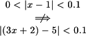
For example, suppose we wish to investigate the assertion
${\displaystyle \lim_{x\rightarrow 1}3x+2=5}$.
Consider the challenge $\varepsilon=0.1$.
In this case choosing $\delta=0.1$ constitutes an
inadequate response.
There are inputs (e.g. $x=1.05$) within $\delta=0.1$
of $x_0=1$ that produce outputs (for $x=1.05$, the
output $f(x)=3(1.05)+2=5.15$) that are not
within $\varepsilon=0.1$ of $L=5$.
But $\delta=0.03$ is an adequate response, since
$0<|x-1|<0.03 \implies 3|x-1|<0.09 \implies |3x-3|<0.09 \implies |(3x+2)-5|<0.09 \implies |(3x+2)-5|<0.1$.
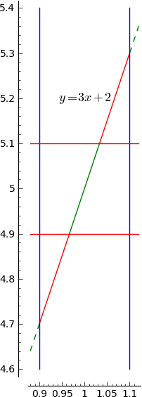
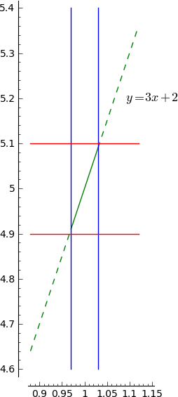
Let's look at this from a graphical perspective.
An $\varepsilon$ challenge sets up upper and lower boundaries at $y=L\pm\varepsilon$.
The $\delta$ response establishes left and right boundaries at $x=x_0\pm\delta$.
If any part of the graph of $y=f(x)$ between the left and right boundaries
(excepting possibly a single point corresponding to input $x_0$ exactly)
fails to stay within the upper and lower boundaries, then the $\delta$ response
is inadequate.
On the other hand, if the portion of the graph of $y=f(x)$ between the left and
right boundaries ($x=x_0\pm\delta$) does indeed stay within the upper and lower
boundaries ($y=L\pm\varepsilon$) (except possibly for a single point $(x_0,f(x_0))$),
then the $\delta$ response is adequate.
The plots immediately below illustrate both the inadequate and adequate responses
to the example challenge described above.
|
|
|
|
|
|
|
So what do we know about a limit assertion after we've determined the "status" (adequate or inadequate) of a particular $\delta$ response to a particular $\varepsilon$ challenge? Frankly, not much. Just because a certain $\delta$ response is inadequate doesn't guarantee that every possible response to the $\varepsilon$ challenge under consideration will surely be inadequate. Perhaps (as in the illustration above) simply chosing a smaller $\delta$ will do the trick. On the other hand, if we've found an adequate response to a particular challenge, that doesn't guarantee that there can't be a stiffer challenge (namely one with a smaller $\varepsilon$) that turns out to be a stumper. In our informal terminology, a limit assertion boils down to a claim that every challenge has an adequate response. Or graphically, no matter how tightly we squeeze the horizontal boundaries close to $y=L$, it's possible to squeeze the vertical boundaries close enough to $x=x_0$ so that the portion of the graph inside the vertical markers stays inside the horizontal ones (again, with the possible exception of one point with $x=x_0$). (This is not at all the same as claiming that every possible response to any challenge will be adequate... or that the graph between vertical markers will stay inside given horizontal markers no matter how widely the vertical markers are spaced.) Since there are always infinitely many possible $\varepsilon$ challenges, we can never show that they all have adequate responses by analyzing them one at a time. So what do we do?
Reconsider our sample limit assertion ${\displaystyle \lim_{x\rightarrow 1}3x+2 = 5}$. And, in particular, look at the condition imposed on values of $3x+2$ by an $\varepsilon$ challenge. This condition is $|(3x+2)-5|<\varepsilon$. Let's not look at any particular values of $\varepsilon$ but rather figure out in terms of $\varepsilon$ which values of $x$ will satisfy the condition. Since $|(3x+2)-5|<\varepsilon \iff |3x-3|<\varepsilon \iff 3|x-1|<\varepsilon \iff |x-1|<\frac{\varepsilon}{3}$ we see that inputs within $\frac{\varepsilon}{3}$ units of the approach point $1$ will always produce outputs $3x+2$ that differ from the proposed limit $5$ by less than the tolerance $\varepsilon$. In other words, we've discovered a strategy for producing an adequate $\delta$ response to any $\varepsilon$ challenge. Simply letting $\delta = \frac{\varepsilon}{3}$ (or anything smaller, but still positive) will always work. A limit proof "from the definition of limit" is essentially a specification of a strategy (a formula for $\delta$ in terms of $\varepsilon$) together with a demonstration that the strategy works (i.e. produces an adequate $\delta$ response to any $\varepsilon$ challenge). So we already have all the pieces for a proof (from the definition of limit) that ${\displaystyle \lim_{x\rightarrow 1}3x+2 = 5}$. Assembling these pieces into a conventional format yields:
| Claim: | ${\displaystyle \lim_{x\rightarrow 1}3x+2 = 5}$. | |||
| Proof: | Let $\varepsilon>0$. | |||
| Choose ${\displaystyle \delta=\frac{\varepsilon}{3}}$. | ||||
| Then $0<|x-1|<\delta$ | ${\displaystyle \implies 0<|x-1|<\frac{\varepsilon}{3}}$ | by definition of $\delta$ | ||
| ${\displaystyle \implies |x-1|<\frac{\varepsilon}{3}}$ | by conjunction elimination | |||
| ${\displaystyle \implies 3|x-1|<3\frac{\varepsilon}{3}}$ | since scaling by a positive preserves inequality | |||
| ${\displaystyle \implies |3x-3|<\varepsilon}$ | by a basic property of absolute value and the distributive rule | |||
| $\implies |(3x+2)-5|<\varepsilon$ | by basic properties of arithmetic | |||
| $\square$ |
Admittedly some of the steps in this proof are so simple
it's a bit anal to give explicit justifications for each step.
But in general it's important to realize that justifications
are essential to proofs.
More importantly, notice that the function involved in this
example limit is particularly simple -- it's linear.
In our preparatory work we easily connected our starting
inequality $|f(x)-L|<\varepsilon$ to something of the form
$|x-x_0|<$expression-in-$\varepsilon$
via a sequence of bi-implications.
Since the proof needs to argue from
$0<|x-x_0|<\delta$ to $|f(x)-L|<\varepsilon$
we don't really need bi-implications in our
preparatory ("scratch") work. But mere forward implications
in the scratchwork in this approach are useless. It's
the reverse implications in the scratchwork that will
"go the right way" when we put together the proof.
This point is important to keep in mind when tackling
trickier limit proof problems.
The Sage Cell below lets you experiment graphically with $\varepsilon$ challenges and $\delta$ responses. Portions of the graph of $y=f(x)$ that are between $x=x_0-\delta$ and $x=x_0+\delta$ but outside the bounds $y=L-\varepsilon$ and $y=L+\varepsilon$ are plotted in red highlighting the inadequacy of the current $\delta$ response to the current $\varepsilon$ challenge. (Assuming you don't change the Sage code the function $f$ you'll be investigating is defined by $f(x)=x\sin{\frac{1}{x}}$, and the approach point $a=0$.)