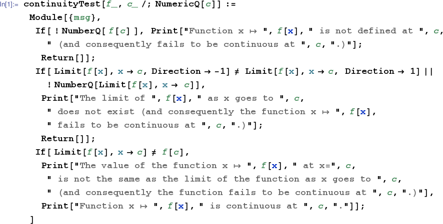
Function $f$ is continuous at $c$ if the following three conditions are satisfied.
(1) $f$ is defined at $c$ (i.e. $f(c)$ exists).
(2) ${\displaystyle \lim_{x\rightarrow c}f(x)}$ exists.
(Equivalently the right and left-hand limits of $f$ at $c$
both exist and equal each other.)
(3) The limiting value and function definition agree at $c$
(i.e. ${\displaystyle \lim_{x\rightarrow c}f(x)=f(c)}$).
(Note that this definition may be modified to define continuity at an endpoint of the domain of a function.)
The code in the first Mathematica subsection below attempts to determine whether or not a given function is continuous at a given point by directly checking the three conditions listed above.
One important corollary of the Intermediate Value Theorem for Continuous Functions guarantees that if a continuous function changes sign on an interval then it has at least one zero on the interval. Routines for approximating zeros numerically are introduced on this page.
The continuous function $f:\mathbb{R}\rightarrow\mathbb{R}$ given by $f(x)=\cos{(3\sin{x})}$ changes sign on the interval $[0,1]$ and thus must have a zero in this interval. The fzero() command may be used to find an approximation to such a zero. One allowable syntax is fzero(function-handle, [xmin xmax]). Notice that the first input to fzero is a function handle. We can pass fzero a handle to an implementation of our example function $f$ as an anonymous function.
octave:1> fzero( @(x) cos( 3*sin(x) ), [0 1] ) ans = 0.55107
Alternatively,
octave:1> fh = @(x) cos( 3*sin(x) ); octave:2> fzero( fh, [0 1] ) ans = 0.55107.
If we implement $f$ as an M-file with contents
function y = f(x) y = cos( 3*sin(x) );
name f.m and storage location somewhere on MATLAB's
path, then, in MATLAB's command window, we can create a handle to
this function with an ampersand.
The function name f and the handle created with
@f are not interchangeable.
octave:1> fzero( @f, [0 1] ) ans = 0.55107 octave:2> fzero( f, [0 1] ) error: `x' undefined near line 2 column 16 error: evaluating argument list element number 1 error: evaluating argument list element number 1 error: called from: error: /home/rsmyth/.octave/f.m at line 2, column 3 error: evaluating argument list element number 1
Note that it's usually advisable to choose longer more descriptive names for functions implemented in M-files.
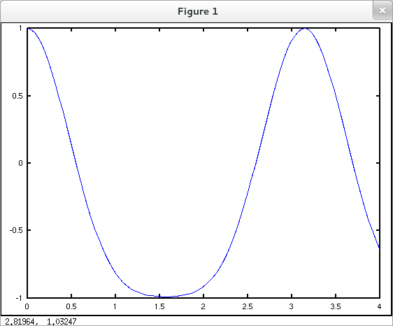
From the graph
octave:1> x = linspace( 0, 4, 100 ); octave:2> y = cos( 3*sin(x) ); octave:3> plot( x, y )
it appears that $f$ has three zeros on the interval $[0, 4]$. Although a single invocation of fzero using the interval specification [0 4] will not return approximations to all three zeros, we can call fzero three times successively using intervals appropriate to each zero. The graph can be used as a guide to find intervals where $f$ changes sign and has (at least apparently) only one zero.
octave:4> fh = @(x) cos( 3*sin(x) ); octave:5> fzero( fh, [0 4] ) ans = 0.55107 octave:6> fzero( fh, [0 1] ) ans = 0.55107 octave:7> fzero( fh, [2 3] ) ans = 2.5905 octave:8> fzero( fh, [3 4] ) ans = 3.6927
If you want to approximate a zero of a function like cosine for which MATLAB has a builtin implementation, then
octave:1> fzero( @(x) cos(x), [0 2] ) ans = 1.5708
is correct, but unnecessarily verbose. The more concise
octave:2> fzero( @cos, [0 2] ) ans = 1.5708
is preferable. But again the ampersand is not optional.
octave:3> fzero( cos, [0 2] ) error: Invalid call to cos.
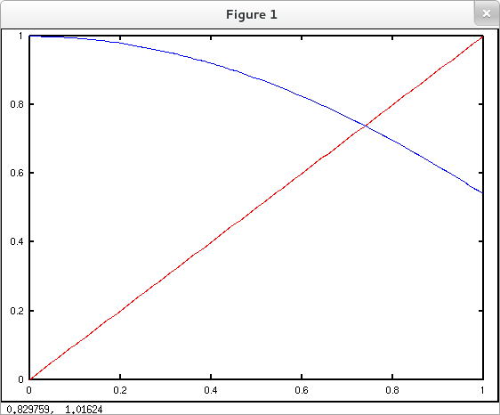
Now suppose you wish to find an approximate solution to an equation such as $\cos{x}=x$. Although at a glance this may appear to be a different ball game, it's trivial to recast the equation as $\cos{x}-x=0$. More generally, $f(x)=g(x)$ is equivalent to $f(x)-g(x)=0$. So equation solving may always be recast as zero hunting. Since the function that maps real numbers $x$ to $\cos{x}-x$ is continuous (everywhere) and changes sign on the interval $[0, 1]$ there must be a zero of this function in $[0, 1]$. That is to say, the equation $\cos{x}=x$ has a solution in $[0, 1]$, and we may compute an approximate solution with fzero.
octave:1> fzero( @(x) cos(x)-x, [0 1] ) ans = 0.73909
Compare this result to the graph below.
octave:2> x = linspace(0,1,100); octave:3> plot( x, x, 'r', x, cos(x), 'b' )
The general purpose routine fzero may of course be used with polynomial functions. However, if you're working with polynomials you should consider using the more specialized roots command. (See the documentation at www.mathworks.com/help/matlab/ref/roots.html.)
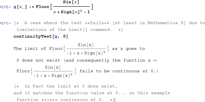
The following continuity test relies essentially on Mathematica's Limit[] command. Since there are some limits this command can't handle, the continuity test is not infallible.
The test.
A few successful trials.
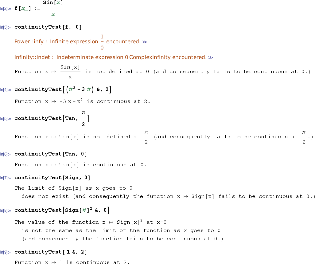
A failure.
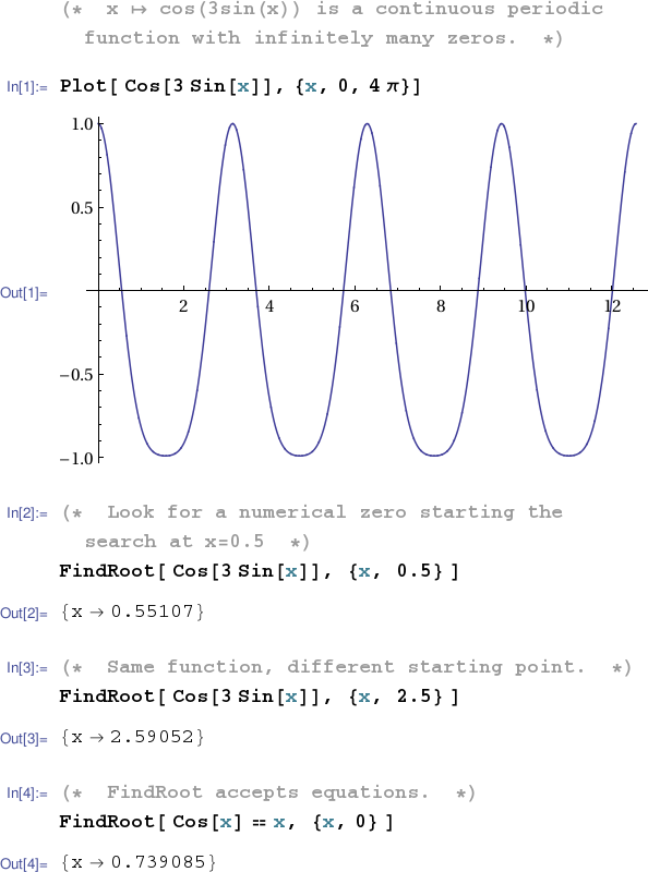
The following notebook illustrates Mathematica's FindRoot[] command.
The cell below illustrates Sage's find_root command. See www.sagemath.org/doc/reference/numerical/sage/numerical/optimize.html for more information.